Exchange 2019 is your ticket to streamlined communication and collaboration. With this comprehensive guide, we'll empower you to master the setup process, ensuring your organization's emails flow effortlessly. 

It's time to elevate your email game and embrace the future of messaging. Let's embark on this transformative journey together.

Table of Contents

1. Prerequisites for Exchange 2019 Setup
2. Planning Your Exchange 2019 Deployment
3. Importance of Planning
4. Installation Process
5. Configuration and Optimization
6. Email Migration to Exchange 2019
7. Backup and Recovery Strategies
8. Security and Compliance
9. Final Thoughts

Prerequisites for Exchange 2019 Setup

Setting up Exchange 2019 requires a few essential components and preparations to ensure a smooth installation process. Let's break it down in simple terms:

1. System Requirements:

• Your server needs to meet specific hardware and software criteria to run Exchange 2019 effectively.
• This includes having a 64-bit processor, sufficient RAM (usually 128 GB or more), and ample storage space. Exchange 2019 also works best on Windows Server 2019.

2. Adequate Hardware Resources:

• Hardware resources like CPU, RAM, and storage are crucial. Exchange is a robust application that handles email communication, and it needs the power to do so.
• If your hardware isn't up to par, Exchange might run slowly, and users may experience delays in email processing.

3. Necessary Software Installations:

• Before installing Exchange 2019, make sure you have certain software in place.
• You'll need .NET Framework 4.8, a software framework by Microsoft that helps Exchange run smoothly.
• Additionally, you should install the Remote Tools Administration Pack using a PowerShell command, which allows you to manage Active Directory Domain Services (ADDS).

Here's a simplified breakdown of the software requirements:

• .NET Framework 4.8: Think of this as the foundation that Exchange stands on. It ensures Exchange has the necessary tools to function properly.
• Remote Tools Administration Pack: This is like the control panel for managing user accounts and permissions within Exchange. It's crucial for setting up user access and control.

Planning Your Exchange 2019 Deployment

Before diving into the installation of Exchange 2019, it's crucial to plan your deployment carefully. This strategic groundwork ensures that your email system runs smoothly and efficiently. Here's why planning is so important and what you should consider:

Importance of Planning

Think of planning as the blueprint for your Exchange setup. It's like mapping out your route before embarking on a road trip; without it, you might get lost.

Planning helps you avoid common pitfalls, reduces downtime, and ensures that your Exchange environment aligns with your organization's needs.

1. Determining Server Roles (HUB, CAS, Mailbox):

• In Exchange, different roles perform distinct functions. Understanding these roles is essential.
• The HUB role manages email traffic, the CAS role handles client access, and the Mailbox role stores emails.
• Deciding which roles your organization needs depends on its size and requirements.

1. Considering High Availability and Scalability:

• High availability ensures your email system remains accessible even if a server goes down.
• Scalability allows your system to grow as your organization does.
• Both factors are vital for uninterrupted email services and future-proofing your setup.

Now, let's simplify the installation steps:

Step 1: Install Windows Server 2019

• This is like setting up the foundation for your Exchange house. Windows Server 2019 provides the operating system for Exchange to run on.

Step 2: Install Prerequisites for Microsoft Exchange 2019 Mailbox Server

• Think of this as gathering all the necessary tools and materials before building something. Exchange needs specific software components to function correctly.

Step 3: Install Exchange 2019 Server

• Finally, this is like assembling the Exchange machinery itself. You're putting together all the parts to create your email system.

Installation Process

Installing Exchange 2019 involves several steps to get your email system up and running. Let's break it down in a straightforward manner:

1. Preparing Active Directory:

• Think of Active Directory as a phonebook for your organization. You need to ensure it's ready to work seamlessly with Exchange.
• This step involves configuring your network settings, permissions, and user accounts to integrate smoothly with Exchange.

2. Installing Exchange Roles:

• Exchange consists of different roles, each serving a specific function.
• During this step, you'll choose which roles to install, such as Mailbox, Client Access, or Edge Transport, depending on your organization's needs.
• It's like customizing your Exchange setup to match your requirements.

3. Configuring DNS and Certificates:

• DNS (Domain Name System) acts as a translator, helping computers find each other on the internet.
• You'll configure DNS settings to ensure your Exchange server's domain name is correctly associated with its IP address.
• Certificates are like digital ID cards for secure communication. You'll set up SSL certificates to protect data transmission.

4. Post-Installation Tasks:

• After the installation, there are essential tasks to wrap things up:
• Configuring email policies and settings.
• Setting up user accounts, mailboxes, and distribution lists.
• Testing the system to ensure everything works smoothly.
• Implementing backup and recovery strategies to safeguard your email data.

Configuration and Optimization

Configuring and optimizing Exchange 2019 is like fine-tuning a race car to ensure it performs at its best. Here's how to do it in simple terms:

1. Enhancing Performance:

• Switch to High-Performance Power: This is like setting your computer to "Turbo Mode" to get the most speed and efficiency.
• Disable DOS 8.3 Short File Names: It's like clearing unnecessary clutter from your workspace for faster access.

2. Monitoring Resources:

• Check for CPU or RAM Consuming Processes: Imagine keeping an eye on which apps are hogging your computer's memory and processing power. You'll manage and optimize accordingly.
• Scan for Malware: Think of this as checking for unwanted intruders in your system. Malware can slow things down, so regular scans are essential.

3. Network Optimization:

• Check Network Speeds: Just like ensuring the roads are clear for a smooth drive, you'll want to ensure your network connections are running at optimal speeds.
• Update Relevant Drivers: Think of drivers as the software that helps your hardware communicate. Keeping them up-to-date is like fine-tuning your engine.

4. Security Measures:

• Check for Signs of Attack: It's like locking your doors and windows. You'll want to monitor your system for any unusual activity or potential threats.
• Disable SMB Packet Signing: This is akin to removing unnecessary security checks at a toll booth to speed up traffic, but it should be done cautiously.

Mailbox and Recipient Policies:

• Configuring mailboxes is like assigning offices to employees. You'll set up email accounts and define who gets access to what.
• Recipient policies are like company rules. You'll establish guidelines for email addresses and distribution.

Performance and Security Settings:

• Optimizing performance settings is like adjusting your car's engine for maximum efficiency. You'll tweak settings to ensure Exchange runs smoothly.
• Security settings are like adding locks to your email doors. You'll configure settings to protect your email system from threats.

Client Access Configuration:

• This is like designing the entrance to your office building. You'll set up how users access their emails, whether through a web browser, mobile app, or desktop client.

Email Migration to Exchange 2019

Migrating emails to Exchange 2019 is akin to transferring your possessions to a new home. Here's a simplified guide:

1. Domain Verification:

Just like ensuring you have the keys to your new house, verify that you own the domain you want to migrate.

2. Connect to Microsoft 365 or Office 365:

Think of this as setting up a secure bridge between your old and new email systems.

You'll connect Exchange 2019 to your Microsoft 365 or Office 365 account.

3. Create Migration Batch:

Imagine packing up your belongings into boxes. In this step, you create a batch that contains all your emails.

This batch is like a moving truck for your emails.

4. Start the Migration Batch:

Just as you'd load your moving truck and set off to your new home, you initiate the email transfer.

Emails from your old system start moving to Exchange 2019.

5. Route Email to Microsoft 365 or Office 365:

It's like updating your postal address with the post office. You'll redirect incoming emails to your new Exchange 2019 server.

6. Delete the Migration Batch:

Once all your emails have safely arrived in Exchange 2019, you can discard the empty moving boxes, which in this case, are the migration batches.

Guide on Email Migration:

If you're transitioning from an old system, we've got you covered with a step-by-step guide.

Options and Tools:

We'll explore various methods and tools available for email migration, helping you choose what suits your needs best.

Troubleshooting Migration Issues:

Just like roadblocks during a move, we'll discuss common migration problems and how to overcome them.

Backup and Recovery Strategies

Backing up your data is like creating a safety net for your digital world. Let's break down why it's crucial and how to do it with Exchange 2019:

1. The Importance of Data Backup:

• Think of data backup as insurance for your emails. Accidents, hardware failures, or cyber threats can happen anytime, and losing critical email data can be disastrous for any organization.
• Regular backups ensure that if the worst does occur, you can quickly recover lost data, minimizing downtime and disruptions.

2. Setting up Backup Solutions:

Setting up backups for Exchange 2019 is like creating a copy of your important files. Here's how:

• Start Windows Server Backup, just like opening a backup app.
• Select "Local Backup" to choose where you want to store your backup.
• Use the "Backup Once" option to initiate a manual backup.
• On the "Backup Options" page, select "Different options" to customize your backup preferences.

3. Recovery Procedures:

Imagine you've misplaced something important, and now you need to find it. In case of data loss, you'll follow these steps:

• Identify the specific data or emails you need to recover.
• Use your backup solution to restore the lost data.
• Carefully follow the recovery process, making sure to select the correct backup point.
• Once the data is restored, your emails and information are back where they belong.

Security and Compliance

Securing Exchange 2019 is like locking the doors to your digital office. Let's understand why it's vital and how to ensure compliance while following best practices:

1. Importance of Securing Exchange:

• Exchange Server allows users to access emails and collaborate across various devices. However, this convenience also makes it a potential target for cyber threats.
• Securing Exchange is critical to protect sensitive data and maintain the integrity of your organization's communication.

2. Compliance with Data Protection Regulations:

• Data protection regulations like GDPR and HIPAA require organizations to safeguard user data. Exchange must adhere to these rules.
• Measures include encrypting emails, ensuring secure access, and implementing policies for data retention and deletion.

3. Security Best Practices:

• Exchange Server 2019 has two main roles: Mailbox and Edge Transport. The Mailbox role handles emails, databases, and client access, while the Edge Transport role focuses on anti-spam and mail flow rules.
• On the client side, Exchange 2019 enhances security with features like calendar forward blocking, out-of-office support, and internationalized email addresses.

Final Thoughts

In wrapping up our journey through setting up Exchange 2019, let's recap the key takeaways. We've learned that meticulous planning is the cornerstone of a successful deployment, ensuring that your email system aligns perfectly with your organization's needs. 

From configuring server roles to optimizing performance, each step contributes to a well-oiled Exchange machine.

One more thing

If you have a second, please share this article on your socials; someone else may benefit too. 

Subscribe to our newsletter and be the first to read our future articles, reviews, and blog post right in your email inbox. We also offer deals, promotions, and updates on our products and share them via email. You won’t miss one.

Related Articles 

» How to Secure Your Servers: A Step by Step Guide
» Fixed: Unable To Shutdown Due to DDE Server Window (explorer.exe)
» How to Download Windows Server 2022

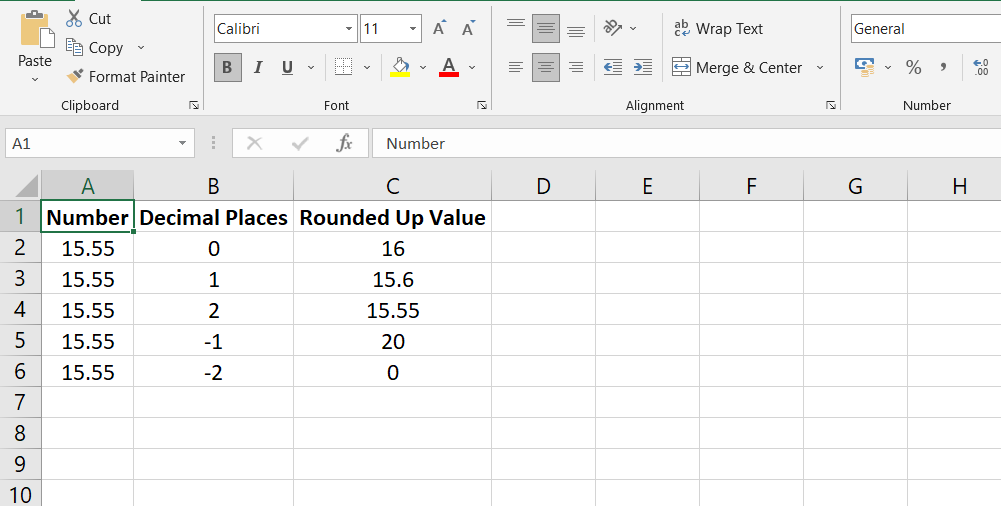
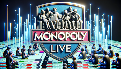
Monopoly Live transforms family game night by letting you play a fast-paced game of Monopoly online with players around the world. Rolls of the dice and movement around the board are automated while a live video dealer interacts with players. Read about Evolution Gaming Monopoly Live to discover the gameplay rules, the software behind it, strategies for outsmarting opponents, and how to play it with friends for maximum fun. Whether you’re a seasoned real estate mogul or new to the game, this guide will help you get started with Monopoly Live.

How Monopoly Live Transforms the Classic Board Game Experience

Monopoly Live takes the beloved Monopoly board game and brings it to life online with a real human dealer. Players join a live video stream and play Monopoly with others from around the world, rolling real dice and moving virtual tokens around an animated game board.

Unlike the offline board game, Monopoly Live allows you to play a quick game anytime without needing to set up the physical board and pieces. The video stream and multiplayer setup make it easy to play with friends or make new ones. The live dealer also helps move gameplay along at a brisk pace.

Key features that enhance the classic Monopoly gameplay include:

• Live HD video stream with a real human dealer
• Multiplayer online play with players around the world
• Animated 3D game board, tokens, and cards
• Chat feature to talk with other players
• Fast gameplay with automated dice rolling
• Ability to play short or long games as desired

Overall, Monopoly Live delivers the fun social dynamics of the traditional board game in a fresh, convenient online format. It’s an excellent option for anyone who wants to experience Monopoly in a new way or play a quick game with friends.

The Rules of Monopoly Live

Monopoly Live casino game follows most of the standard official Monopoly rules, with a few adaptations to translate gameplay online. Here are the key rules:

Starting a Game:

To begin a game, players select their virtual token and enter the dollar amount they want to play for. The minimum bet is usually around $1. The dealer shuffles the deck and deals out the properties around the board.

Taking Turns

On a turn, a player rolls two dice with the click of a button and moves their token clockwise around the board that number of spaces. Different actions occur depending on which space a player lands on:

• Property: If unowned, the player can choose to purchase it for the listed price. If owned by another player, they must pay rent.
• Chance/Community Chest: Draw a card and follow its instructions.
• Income Tax: Pay a percentage of the total worth.
• Jail: Just visiting sends the player back to the previous spot. Landing here results in being sent to jail.
• Free Parking: No action.
• Go To Jail: The player is sent directly to jail.

Winning the Game

The goal is to drive opponents into bankruptcy by buying properties and collecting rent. If a player runs out of money, they are eliminated. The last player remaining wins.

Software Behind Monopoly Live

Monopoly Live is powered by innovative real-time gaming software to enable the online multiplayer experience. Key technical elements include:

• Video streaming - The dealer and game board are captured and broadcast in a live HD video stream. This allows players to follow gameplay as it happens.
• Animated game engine - The board, tokens, cards, and other elements are rendered in real-time 3D animation for an immersive experience. Actions like dice rolls and token moves are automated.
• Multiplayer connectivity - Players join from a desktop or mobile in a shared lobby. The software enables real-time chat and seamless gameplay across geographies.
• Randomization - Actions like card draws and dice rolls leverage server-side randomization to ensure fair results.
• Scalability - The games are hosted on cloud infrastructure that can scale to support thousands of simultaneous players across multiple tables.

This blend of video streaming, animation, connectivity, and randomness comes together to make Monopoly Live feel like you're playing the board game through your screen.

Starting a Game of Monopoly Live

Getting started with Monopoly Live is quick and easy:

Set Up the Game Space

The game video stream will be your board, so make sure you have a clear view of your screen without too many distractions in the background. Having a stable internet connection is also recommended.

Choose Your Token

When you join a table, you'll be prompted to select a virtual token - the top hat, car, dog, and more. This token will represent you on the board.

Fund Your Bank

Add money to your virtual wallet to use for bets, property purchases, and rent payments during the game. The minimum bet is usually $1.

Wait for Other Players

Once you've joined a table, it may take a minute or two for other players to fill the remaining spots. The dealer will greet new players as they join.

Let the Dealer Shuffle and Deal

When all player spots are filled, the dealer will shuffle the deck and place the cards face down around the board. Then the fun begins!

Taking Turns in Monopoly Live

Gameplay in Monopoly Live progresses with players taking turns:

• Roll the Dice

Click the dice roller button to instantly roll and get your movement number for the turn. The dealer will also roll physical dice on the camera for added realism.

• Move Your Token

Your token will automatically move around the board with the corresponding number of spaces. Pay attention to which space you land on.

• Perform Actions

Follow the rules of whatever space you land on - pay rent, draw a card, purchase a property, etc. The dealer will walk you through any actions.

• Pass Go

If you pass Go, collect $200! This added money will help you purchase more properties.

• Next Player's Turn

Once your actions are complete, the next player takes their turn and rolls the dice. The gameplay continues until one player goes bankrupt.

Strategies for Winning at Monopoly Live

Use these proven tips and tactics to improve your chances of dominating a Monopoly Live game:

Buy Properties Strategically

The key path to victory is purchasing properties and collecting rent from opponents. Focus early on buying sets of properties that are more likely to be landed on and quickly build houses to increase rent. The light blue and orange sets are cost-effective investments.

Make Smart Trades

If another player has a monopoly you need to complete your own, try trading with them. Sweeten the deal by offering cash or getaway rent-free cards in addition to property.

Don't Overspend Early

Avoid depleting your cash reserves too early through reckless auctions or purchases. Save money to have flexibility later for bidding wars and development.

Know When to Develop

Don't rush to put houses on each property you own. Wait until you have the rent-generating potential to recoup the investment quickly.

Take Smart Risks

An occasional risky investment like an auction bid can pay off, but don't make a habit of it. Calculate odds of success before taking on risk.

Use Get Out of Jail Cards

Hang onto Get Out of Jail Free cards as long as possible. They come in very handy later when you're accumulating rent-generating monopolies.

With the right balance of luck and these Monopoly Live strategies, you'll be on the path towards outplaying your opponents and dominating the online leaderboards!

Playing Monopoly Live with Friends

One of the best parts of Monopoly Live is being able to play with friends and chat while you compete. Here's how to set up and enjoy multiplayer games:

Set Up a Private Game

For the most control, you can reserve a private table and then invite friends to join you. This ensures you play together.

Share a Game Link

Once you're set up in a game, copy the unique table URL and share it with friends. They can use the link to join you directly.

Chat During the Game

The live chat feature lets you trash talk, negotiate trades, or just catch up with friends while playing. It adds to the social fun.

Form Alliances

You can collaborate by forming property-trading alliances with one or two other players. This can increase your collective negotiating leverage against the other players.

See Who Dominates

Play a series of games in one sitting and see who can win the most or earn the highest overall bankroll. Tallies help you determine the true Monopoly master among your group of friends.

While you play to win, having friends in the game makes it a more enjoyable journey!

Bottom Line

Monopoly Live succeeds in bringing all the strategic excitement of the classic board game into a fresh online format perfect for today's digital lifestyles. With a real human dealer, slick animations, multiplayer support, and lively chat, it provides an engaging and competitive environment.

The ability to play on-demand and the accelerated pace make Monopoly Live ideal for quick sessions with friends or making new gaming connections. Succeeding takes equal parts luck, negotiation skills, and investment strategy - a compelling blend. While passing Go and collecting $200 will always be thrilling, Monopoly Live ups the ante for the digital age.

Com instruções fáceis de usar e ferramentas de conversão gratuitas, você está a poucos minutos de um fluxo de trabalho mais tranquilo e produtivo. Mergulhe agora para desbloquear o poder das conversões fáceis de PDF em Google Doc e revolucionar sua experiência de gerenciamento de documentos.

Índice

1. Por que converter PDF em Documento Google
2. Como converter PDF em Documento Google
3. Ferramentas on-line para conversão sem esforço
4. Dicas para uma conversão bem-sucedida
5. Considerações Finais

Por que converter PDF em Documento Google

PDFs são como instantâneos imutáveis ​​de documentos. Embora sejam ótimos para compartilhar informações em um formato fixo, eles podem ser teimosos quando você precisa fazer alterações.

Imagine que você não pode ajustar uma frase, adicionar uma nota ou alterar uma imagem em um PDF que você não criou - é aí que começa a frustração. É aqui que o Google Docs entra para salvar o dia.

1. Mantenha a formatação com liberdade de edição:

Quando você converte um PDF em Documento Google, é como transformar uma imagem em um quebra-cabeça que você pode reorganizar. Seu layout original permanece intacto, as fontes mantêm seu estilo e as imagens permanecem no lugar. Mas agora você não está apenas olhando para isso – você está realmente no controle.

Palavras, parágrafos e imagens podem ser movidos, ajustados ou substituídos sem quebrar a harmonia visual.

2. Modo Ninja Colaborativo:

Imagine uma sala de reuniões virtual onde você e sua equipe editam um documento juntos, onde quer que estejam. Esse é o Google Docs.

Quando um PDF se torna um Documento Google, a mágica acontece. Várias pessoas podem participar, adicionar suas ideias, fazer alterações e ver tudo em tempo real. Chega de cadeias intermináveis ​​de e-mails ou arquivos indo e voltando.

É como ter um playground compartilhado onde todos podem construir o mesmo castelo de areia.

3. Acesso a qualquer hora e em qualquer lugar:

Aqui está a parte legal: o Google Docs está on-line. Contanto que você tenha internet, você tem acesso.

Não há necessidade de carregar pen drives ou anexos de e-mail. Esteja você no computador do trabalho, no laptop do seu amigo ou até mesmo no telefone esperando na fila para tomar um café, basta abrir um navegador e pronto, aí está o seu documento, pronto para editar.

Como converter PDF em Documento Google

Converter um PDF em um Documento Google não é um truque de mágica; é como transformar um tipo de documento em outra versão mais flexível. Você pode fazer isso diretamente no Google Drive, onde guarda todos os seus itens digitais.

1. Mantenha o PDF à mão:

Primeiro, tenha o PDF que deseja imprimir em seu computador. Talvez seja um artigo, um relatório ou algumas notas – seja o que for, certifique-se de que seja fácil de encontrar.

2. Diga oi para o Google:

Tem uma conta do Google? Perfeito. Basta fazer login nele. O Google Drive é como sua sala de armazenamento digital, e o Google Docs é uma das ferramentas dessa sala.

3. Faça upload do PDF:

Ok, agora o PDF precisa entrar na nuvem do Google a partir do seu computador. Pense nisso como enviar um pacote pela internet. Clique no botão "Upload", localize seu PDF e deixe-o fazer seu trabalho.

4. O passo mágico: abrir com o Google Docs:

Você vê aquele PDF no seu Google Drive? Clique com o botão direito nele e um pequeno menu aparecerá. Clique em "Abrir com."Escolha" Documentos Google."

5. Verifique seu novo Documento Google:

Espere um momento enquanto a mágica acontece. O Google transformará seu PDF em um Documento Google. Você verá as palavras, os parágrafos – tudo, exatamente como no PDF. Mas aqui está o melhor: agora é um verdadeiro Google Doc, o que significa que você pode editá-lo, reproduzi-lo e compartilhá-lo como quiser.

Ferramentas on-line para conversão sem esforço

Você já desejou que converter PDFs em Documentos Google fosse tão fácil quanto apertar um botão? Bem, conheça o elenco de ferramentas online que podem fazer isso acontecer. Esses campeões digitais pretendem transformar esses PDFs estáticos em Google Docs dinâmicos sem esforço.

1) PDFSimpli: seu conversor rápido

Este é uma estrela porque não apenas converte, mas também permite editar. PDFSimpli chega com velocidade e simplicidade. Ele transforma seu PDF em um arquivo que você pode inserir diretamente no Google Drive. Mole-mole.

2) LightPDF: o versátil

LightPDF não trata apenas de conversão; é um super-herói PDF. Ele pega qualquer PDF e faz truques de mágica, transformando-o em Word, PPT, Excel e muito mais. Além disso, ele pode editar, compactar, assinar e fazer ainda mais acrobacias com seus documentos.

3) Google Drive: o rosto familiar

Quer o caminho mais simples? O Google Drive é como seu velho amigo de confiança. É onde fica o Google Docs, e adivinhe? Carregar um PDF e convertê-lo em um Documento Google é um passeio no parque.

4) Microsoft Word: a lenda do Office

Provavelmente você já ouviu falar do MS Word. Bem, não se trata apenas de digitar – ele pode lidar com PDFs como um profissional. Abra um PDF no MS Word; ele se transforma em um formato do Google Doc como mágica.

5) EasePDF: a opção fácil e fácil

Como o nome sugere, o EasePDF cumpre sua promessa. Não há ciência de foguetes aqui - basta enviar seu PDF, clicar em um botão e pronto, você tem um Documento Google.

Dicas para uma conversão bem-sucedida

Converter PDFs em Google Docs é como dar uma nova vida aos seus documentos. Mas para tornar a transição perfeita, você precisa manter algumas coisas em mente. Aqui estão duas dicas importantes que tornarão sua jornada de conversão muito fácil.

1) Qualidade é importante:

Pense no seu PDF como uma pintura. Para uma imagem mais clara no Google Docs, comece com um PDF de alta qualidade. O que isso significa? Bem, se o seu PDF tem texto nítido, imagens claras e não é apenas uma imagem (sim, alguns PDFs são assim), você está no caminho certo.

2) Polonês pós-conversão:

Imagine que você está se mudando para um novo lugar – você organizaria as coisas de acordo com seu estilo, certo? Da mesma forma, seu Documento Google pode precisar de um pouco de formatação após a conversão. Verifique títulos, espaçamento, fontes – todos esses detalhes. É como ter certeza de que seu novo espaço parece perfeito.

Considerações Finais

Converter PDFs em Google Docs traz um mundo de vantagens. Trata-se de manter seu layout original e ao mesmo tempo obter o poder de editar e colaborar perfeitamente.

Com formatos mantidos, flexibilidade aprimorada e acessibilidade de qualquer lugar, seu jogo de documentos subiu de nível. Aproveite esta atualização transformadora do fluxo de trabalho e experimente a liberdade dos documentos editáveis.

Torne seu trabalho mais tranquilo, seu trabalho em equipe mais forte e suas ideias mais dinâmicas – tudo com apenas alguns cliques. É hora de transformar esses PDFs estáticos em possibilidades dinâmicas. Mergulhe e aproveite a evolução.

Mais uma coisa

Se você tiver um segundo, compartilhe este artigo em suas redes sociais; outra pessoa também pode se beneficiar.

Assine nosso boletim informativo e seja o primeiro a ler nossos futuros artigos, análises e postagens de blog diretamente na sua caixa de entrada de e-mail. Também oferecemos ofertas, promoções e atualizações sobre nossos produtos e as compartilhamos por e-mail. Você não vai perder nenhum.

Artigos relacionados 

» Importando dados de PDF para Excel: um guia passo a passo
» Como corrigir o recurso Microsoft Print to PDF que não funciona
» Como inserir PDF no Excel

Embarque conosco em uma jornada enquanto nos aprofundamos em quatro ferramentas de IA excepcionais que se destacam na criação de apresentações. Desde interfaces intuitivas até capacidades de design dinâmico, este guia irá iluminar as vantagens distintas de cada opção. Pronto para transformar suas apresentações?

Vamos mergulhar e descobrir o criador de AI PPT que redefinirá sua abordagem para cativar públicos.

Índice

1. O que são criadores de AI PPT?
2. Por que escolher as ferramentas AI PPT Maker?
3. Principais recursos das ferramentas AI PPT Maker
4. Escolhendo a ferramenta AI PPT Maker certa
5. Aproveitando ao máximo as ferramentas AI PPT Maker
6. Considerações Finais

O que são criadores de AI PPT?

Os criadores de AI PPT são ferramentas inovadoras projetadas para simplificar a criação de apresentações impactantes. Apesar dos recursos robustos das ferramentas de produtividade tradicionais, elas geralmente apresentam obstáculos de complexidade. É aqui que entram os fabricantes de AI PPT.

Imagine ter um assistente virtual que entende seu idioma e monta seus slides rapidamente. Essas ferramentas aproveitam algoritmos avançados de IA e ML, aprendendo com as contribuições do usuário para refinar continuamente suas sugestões de design. Você pode escolher entre uma seleção de fontes, planos de fundo e animações sem esforço, economizando tempo e esforço criativo.

Por que você deve considerar o uso de ferramentas de criação de AI PPT? Aqui está o resumo:

1. Criação rápida de design: essas ferramentas produzem modelos, temas e layouts, alinhando-os com a essência e a voz da sua marca, garantindo uma apresentação refinada e consistente.
2. Geração de conteúdo atraente: crie títulos que chamem a atenção, obtenha imagens relevantes e formate slides perfeitamente. Isso ajuda na construção de apresentações persuasivas e visualmente atraentes.
3. Personalização sob medida: refine as apresentações de slides existentes sem esforço, ao mesmo tempo que segue as diretrizes da sua marca. Cada apresentação mantém uma aparência coesa e profissional.

As ferramentas de criação de AI PPT aproveitam o potencial da inteligência artificial para agilizar o design de apresentações. Eles atendem àqueles que buscam eficiência, visuais impressionantes e branding coeso. Essas ferramentas atuam como suas companheiras criativas, facilitando a elaboração de apresentações envolventes sem o incômodo de softwares complexos.

Por que escolher as ferramentas AI PPT Maker?

Optar por ferramentas de criação de AI PPT traz uma série de vantagens que transformam sua experiência de criação de apresentações:

1. Velocidade sem esforço: As ferramentas de criação de AI PPT turbinam o processo de criação de apresentações. Pense nisso como ter um copiloto confiável. Eles simplificam cada etapa, ajudando você a criar slides envolventes em uma fração do tempo que normalmente levaria.
2. Excelência Visual: Com essas ferramentas, você pode acessar um tesouro de elementos de design avançados. Imagine ser capaz de criar um logotipo tendo um designer experiente oferecendo sua experiência. Seu visual se torna refinado, cativando seu público com seu talento profissional.
3. Harmonia de formatação: Um dos desafios mais significativos no design de apresentações é manter a formatação e o layout consistentes. As ferramentas do AI PPT Maker são como seus anjos da guarda de formatação. Eles garantem que cada slide siga o estilo escolhido, criando uma aparência coesa e elegante.

Imagine ter um assistente de apresentação que acelera o processo e eleva a qualidade dos seus slides. As ferramentas do criador de AI PPT não são apenas uma questão de conveniência; o objetivo é transformar suas apresentações em ferramentas de comunicação poderosas com o mínimo de esforço.

Portanto, seja você um apresentador experiente ou novo no jogo, essas ferramentas estão à sua disposição, fazendo suas apresentações brilharem e deixando um impacto duradouro em seu público.

Principais recursos das ferramentas AI PPT Maker

As ferramentas de criação de AI PPT são o seu segredo para criar apresentações impressionantes com facilidade. Essas ferramentas aproveitam tecnologia de ponta para aprimorar o processo de criação de apresentações. Vamos explorar alguns de seus recursos mais destacados e como eles podem beneficiar você:

1. Interface de usuário intuitiva:

Imagine ter uma ferramenta que o guia sem esforço pelo processo de criação de apresentações. Os fabricantes de AI PPT são projetados tendo em mente a facilidade de uso. Navegar pelos modelos, adicionar conteúdo e personalizar layouts torna-se muito fácil, mesmo para iniciantes.

2. Sugestões de conteúdo com tecnologia de IA:

Imagine ter um parceiro criativo virtual que fornece sugestões personalizadas para slides impactantes. Essas ferramentas analisam seu conteúdo e sugerem recursos visuais, títulos e muito mais. É como ter um assistente de IA ao seu alcance.

3. Extensa biblioteca de modelos:

Pense no incômodo de procurar o modelo perfeito. Com os criadores de AI PPT, você pode acessar uma biblioteca abrangente de modelos, gráficos e ícones. Essa variedade garante que suas apresentações sejam envolventes e visualmente refinadas.

Vamos dar uma olhada em algumas ferramentas notáveis ​​do criador de AI PPT:

Lindo.IA

Esta ferramenta oferece simplicidade sem comprometer recursos. Ele gera slides cativantes em apenas 60 segundos. De uma biblioteca de modelos de apresentação a um gerador de gráficos integrado, o Beautiful.A IA facilita muito a criação de apresentações atraentes.

Microsoft Copilot para PowerPoint

Utilizando o poder do GPT-4, o Microsoft Copilot acelera a geração de ideias e a criação de conteúdo. Embora baseado em assinatura, é a escolha ideal para indivíduos e equipes que buscam economizar tempo e elevar suas apresentações.

WPS AI para apresentação

WPS AI, que em breve será integrado ao pacote Kingsoft Office, promete scripts persuasivos, criação de apresentações de slides sem esforço e colaboração perfeita. É uma ferramenta gratuita com uma extensa biblioteca de modelos, o que a torna uma opção promissora.

Imagem 6

Apresentações IA

Perfeito para usuários do Apresentações Google, o Slides AI simplifica a criação de slides usando prompts de texto. Sua integração com o Apresentações Google garante uma experiência perfeita. Com designs personalizáveis ​​e recursos que economizam tempo, é uma vantagem para quem confia na plataforma do Google.

As ferramentas AI PPT maker redefinem a criação de apresentações, tornando-as acessíveis e eficientes. Quer você seja um apresentador experiente ou novo no cenário, essas ferramentas oferecem uma série de benefícios, desde o aprimoramento visual até a simplificação de todo o processo. Explore essas opções e descubra como a IA pode revolucionar seu jogo de apresentação.

Escolhendo a ferramenta AI PPT Maker certa

Quando se trata de escolher a ferramenta certa para criação de AI PPT, algumas estratégias importantes podem ajudá-lo a navegar pelo cenário com confiança:

1. Avaliações e classificações de usuários são importantes:

Pense nas avaliações e avaliações dos usuários como sua bússola. Esses insights fornecem uma visão real do desempenho de uma ferramenta. Você está aproveitando a experiência coletiva daqueles que o usaram. Procure feedback consistentemente positivo e classificações altas, muitas vezes indicando a confiabilidade e eficácia de uma ferramenta.

2. Adaptando recursos às suas necessidades:

Imagine comprar um terno sob medida - você escolheria um que combinasse perfeitamente com você, certo? Da mesma forma, avalie os recursos das ferramentas do AI PPT maker em relação aos seus requisitos de apresentação. Você precisa de elementos de design avançados? Recursos colaborativos? Certifique-se de que a ferramenta esteja alinhada com o que você imagina para suas apresentações.

Encontrar a ferramenta ideal para criação de AI PPT é uma combinação de verificar as experiências de outros usuários e combinar os recursos da ferramenta com seus objetivos de apresentação. Ao combinar essas abordagens, você estará bem equipado para tomar uma decisão que se alinhe às suas necessidades exclusivas e garanta que suas apresentações realmente se destaquem.

Aproveitando ao máximo as ferramentas AI PPT Maker

Assim como você aprimora uma receita para um prato delicioso, você pode ampliar seus resultados usando ferramentas de criação de AI PPT, implementando estratégias inteligentes que aumentam a criatividade e o engajamento.

1. Maximizando a criatividade e a eficiência:

Pense nessas ferramentas como suas assistentes artísticas. Para aproveitar todo o seu potencial:

• Aplique dicas que aumentem a criatividade e garantam o uso eficiente da ferramenta.
• Estabeleça canais de comunicação eficazes para uma colaboração perfeita.
• Incentive discussões abertas que tragam diversas perspectivas para a mesa.
• Promova um ambiente colaborativo onde as ideias fluam livremente.
• Defina claramente as metas e prazos do projeto para permanecer no caminho certo.

2. Conteúdo personalizado para engajamento:

Agora, considere como o conteúdo personalizado é como adicionar temperos ao seu prato de apresentação:

• Reúna dados de membros para entender melhor seu público.
• Use a segmentação para atingir grupos específicos com mensagens personalizadas.
• Integre questionários interativos para tornar sua apresentação envolvente.
• Aproveite ferramentas como geolocalização por IP para um toque localizado.
• Adicione uma pitada de gamificação para manter seu público envolvido.
• Envie e-mails personalizados que correspondam às preferências individuais.
• Divulgue conteúdo para novos membros, mantendo-os engajados ao longo do tempo.
• Aproveite anúncios redirecionados nas mídias sociais para maior alcance.

Nas ferramentas de criação de AI PPT, dominar a criatividade e o envolvimento é semelhante a criar uma obra-prima. Ao combinar técnicas de aumento de eficiência com estratégias de engajamento personalizadas, suas apresentações irão cativar e deixar um impacto duradouro em seu público.

Portanto, combine o poder das ferramentas de IA com essas táticas e veja suas apresentações atingirem novos patamares de excelência.

Considerações Finais

Abraçar o mundo das ferramentas de criação de AI PPT é um convite à criatividade e eficiência ilimitadas. Essas ferramentas permitem que você crie facilmente apresentações impressionantes, economizando tempo e esforço e, ao mesmo tempo, entregando resultados excepcionais. Ao aproveitar interfaces intuitivas, sugestões de conteúdo baseadas em IA e uma variedade de elementos de design, suas apresentações estão preparadas para cativar e inspirar.

Ao embarcar nesta jornada, lembre-se de que as possibilidades são infinitas. Desde a criação simplificada de design até estratégias de engajamento personalizadas, essas ferramentas oferecem um universo de potencial a ser explorado.

Mais uma coisa

Se você tiver um segundo, compartilhe este artigo em suas redes sociais; outra pessoa também pode se beneficiar.

Assine nosso boletim informativo e seja o primeiro a ler nossos futuros artigos, análises e postagens de blog diretamente na sua caixa de entrada de e-mail. Também oferecemos ofertas, promoções e atualizações sobre nossos produtos e as compartilhamos por e-mail. Você não vai perder nenhum.

Artigos relacionados 

» Os 10 melhores criadores de logotipos gratuitos em 2023
» Como encontrar concorrentes ' Palavras-chave para catapultar seu SEO
» Como imprimir títulos do Excel em todas as páginas | Guia passo a passo

Say goodbye to compatibility issues and hello to polished documents ready for sharing, printing, or archiving. Whether you're a student, professional, or anyone needing to convert Pages to PDF, this guide has you covered. 

Let's dive in and simplify your document conversion process today. 

Table of Contents

1. Methods to Convert Pages to PDF on Windows
2. Pages to PDF Online Converters
3. Steps to Convert Pages to PDF on Mac
4. Print to PDF Method for Converting Pages Documents
5. Best Practices for Converting Pages to PDF
6. Final Thoughts

Methods to Convert Pages to PDF on Windows

Converting your Pages documents to PDF through Microsoft Word is a straightforward process that ensures compatibility and ease of use. Here's a step-by-step guide to help you effortlessly create PDFs from your Pages files.

Open Pages Document in Word

1. Launch Microsoft Word on your Windows computer.
2. Within your Pages document, click on the "File" menu at the screen's top-left corner.

Export Pages Document

1. From the "File" menu, select "Export To."
   
   
   
2. Choose either "PDF..." or "Word..." depending on your preferred output format. If you're uncertain, consider asking for guidance from your instructor.

Save as PDF in Word

1. After exporting, the Pages document will open in Word.
2. Click on the "File" tab at the top-left corner of Word's interface.
3. Select "Save As" and then "Browse" to choose a destination folder.
4. Enter a name for the file in the "File Name" box.
5. From the "Save as type" dropdown, choose "PDF (*.pdf)." 
   
6. If needed, adjust printing and markup options under "Options."
7. Finally, click "Save" to convert and save the document as a PDF.

Converting Pages to PDF using Microsoft Word guarantees that your document's layout remains intact, and it's easily shareable without compatibility concerns. Following these steps, you can efficiently convert your Pages files to PDF format, ready for distribution, printing, or archiving.

Remember to save your Word documents frequently (Ctrl+S), and when you're ready to print, just go to the "File" tab and select "Print." This approach streamlines creating PDFs from Pages documents, making it accessible even for those new to document conversion.

Pages to PDF Online Converters

If you're seeking a speedy online solution to convert your Pages documents to PDF format, several user-friendly tools can do the job effortlessly. These tools come in handy when you don't want to install software or prefer a quick conversion process.

Zamzar

Zamzar offers a free and simple online conversion tool for transforming Pages files into PDFs with just a few clicks. All you need to do is upload your Pages document, choose the PDF output format, and let Zamzar work its magic. It's a straightforward and accessible option for anyone looking to convert without the hassle of downloads.

Adobe

For those familiar with Adobe Acrobat, you can use its "Create PDF" tool to convert web pages or HTML files into PDF format. Simply navigate to Tools > Create PDF > Web Page in Acrobat, enter the web page's path or locate an HTML file on your computer.

pdf2go

pdf2go is another convenient online PDF converter that accepts various file formats, including images, Word documents, spreadsheets, and presentations. This versatile tool lets you easily transform many documents into PDFs, making it useful for various needs.

Pros and Cons of Online Converters

Pros:

• Convenience: No software installation is required; accessible from any device with an internet connection.
• Speed: Swift conversion process for quick results.
• No Compatibility Issues: Online converters often ensure compatibility with different devices and operating systems.

Cons:

• Internet Dependency: Requires an active internet connection for conversion.
• Privacy Concerns: Users should be cautious with sensitive information, as files are uploaded to external servers.

Recommended Tool: 

Among the options, Zamzar stands out for its user-friendly interface and straightforward conversion process. Here's a simple guide to using Zamzar:

1. Visit Zamzar's website.
2. Upload your Pages document.
3. Choose "PDF" as the output format.
4. Enter your email to receive the converted PDF.
5. Click "Convert" and wait for the email with your PDF attachment.

Online converters offer a practical way to convert Pages documents to PDF format without any technical know-how. However, always be mindful of privacy and choose a reputable tool like Zamzar for a seamless and secure conversion experience.

Steps to Convert Pages to PDF on Mac

When it comes to converting Pages documents to PDF format on your Mac, the built-in Pages app offers a straightforward solution. This method ensures both ease of use and preserving your document's integrity.

Using Pages App

The Pages app comes with a handy feature that effortlessly guides you through the process of exporting your Pages document as a PDF. This built-in functionality is not only user-friendly but also maintains the layout and quality of your document.

Exporting as PDF

To convert your Pages document to PDF format using the Pages app:

1. Open the Pages document you wish to convert.
2. From the top menu, select "File" and then "Export To."
3. Choose "PDF" as the export format from the options provided.
4. You can specify additional export settings if needed.
5. Click "Next" and save your PDF file with a suitable name and location.

Converting Pages to Microsoft Word:

If you need to convert your Pages document to Microsoft Word format, follow these steps:

1. Open the desired Pages document.
2. Click on "File" in the top-left corner.
3. Select "Export To" and then choose "Word."
4. Click "Next" and provide a name for your exported Word document.
5. Choose the location where you want to save the file and click "Export."

Converting Pages documents to PDF or Microsoft Word format on your Mac is a breeze using the Pages app. The native features make the process user-friendly, and you have the flexibility to customize your export settings. Whether you share or archive documents, these steps ensure a seamless conversion experience.

Print to PDF Method for Converting Pages Documents

Converting your Pages document to PDF format using the "Print to PDF" method offers an accessible and practical solution. This approach mimics printing a document, making it intuitive for users.

Convert Pages Document to PDF

Converting a Pages document to PDF using the "Print to PDF" method is remarkably straightforward:

1. Open the Pages document you wish to convert.
2. From the "File" menu at the top, select "Export To."
3. Opt for "PDF" as the export format and click "Next."
4. Choose a suitable location to save your PDF and assign a name.
5. Click "Export" to complete the conversion.

Printing a Document from Pages

To print a document from Pages:

1. Open the document in Pages.
2. From the "File" menu, choose "Print."
3. Select a printer from the pop-up menu; if no printers are available, add one via "Add Printer."
4. Adjust print options as needed, like page range or layout.
5. Click "Print" to produce a hard copy.

Printing as a PDF on a Mac

If you'd like to save a document as a PDF on a Mac:

1. Open the document you want to convert in any application.
2. Access the "File" menu and choose "Print."
3. In the print dialog, spot the PDF button or the down arrow next to it.
4. Select "Save as PDF" from the menu.

The "Print to PDF" method simplifies the conversion process by resembling regular printing. This user-friendly and practical technique ensures that even those unfamiliar with document conversion can effortlessly create PDFs. Whether preserving or sharing documents electronically, this method provides a reliable and accessible approach.

Best Practices for Converting Pages to PDF

When converting your Pages documents to PDF format, a few key practices can enhance the quality and professionalism of your final output. These practices ensure that your document appears as intended and effectively communicates your message to the audience.

1. Optimize Images:

Images in your Pages document should be of suitable quality and resolution to avoid pixelation or blurriness in the PDF version. Resize and compress images to maintain clarity while keeping file size manageable.

2. Maintain Fonts:

Use standard fonts that are widely available to ensure consistent rendering across different devices and platforms. Embed fonts in the PDF to preserve the original document's typography and layout.

3. Check Document Layout:

Ensure that the layout, formatting, and alignment of elements remain consistent during the conversion. Elements like headers, footers, tables, and margins should maintain their integrity in the PDF version.

4. Proofread Before Sharing:

Proofreading is crucial before sharing or printing the PDF. Carefully review the content for spelling, grammar, punctuation, and formatting errors. This step ensures that your document is polished and free from mistakes, presenting a professional image to your readers.

Proofreading is a final quality check, enhancing the document's accuracy and effectiveness. It eliminates errors that could hinder comprehension or distract readers from the intended message. Proofreading is the last opportunity to refine the document's quality before it reaches its audience.

Final Thoughts

In conclusion, converting Pages documents to PDF format is a simple yet essential skill for both Windows and Mac users. Whether you're a student, professional, or anyone needing to share documents, the process ensures compatibility, professionalism, and ease of distribution. 

On Windows, using Microsoft Word or online converters like Zamzar offer versatile options, while Mac users can rely on the built-in Pages app or the "Print to PDF" method. Remember to optimize images, maintain fonts, and proofread the PDF before sharing or printing to ensure a polished and error-free document. 

With these straightforward methods at your disposal, you can confidently convert Pages to PDF and streamline your document-sharing process on both platforms.

One more thing

If you have a second, please share this article on your socials; someone else may benefit too. 

Subscribe to our newsletter and be the first to read our future articles, reviews, and blog post right in your email inbox. We also offer deals, promotions, and updates on our products and share them via email. You won’t miss one.

Related Articles 

» Importing Data from PDF to Excel: A Step-by-Step Guide
» How to Fix the Microsoft Print to PDF Feature Not Working

As every business nowadays strives to grow online, investigating online competitors' performance and SEO efforts is essential to paving the way for more customers and sales, and better brand recognition. Finding competitors' keywords should be the first thing on your to-do list when attempting to outrank your niche rivals and lure potential clients.

Unearthing your competitors' SEO strategies and revealing their top-of-mind keywords is a stepwise process that requires precise attention to detail. You should pinpoint your niche competition thoroughly to ensure you're reaching the same target market. 

Moreover, you need to look for the right keywords to implement in your strategy, compile a list of competitor pages relevant to your keyword search, utilize all-around tech tools to get comprehensive competitor data insights, and wisely incorporate the findings into your strategy.

Let this article be your guide to outsmarting the online competition and finding the most valuable and powerful competitor keywords in no time.

3 Primary Steps to Find Competitors’ Keywords

Spying on your competitors' main keyword tactics and discovering their keywords ideas is an exciting yet time and energy-consuming process. Hopefully, the three steps below will serve as a shortcut to unlocking your competitors' keyword strategies.

Step 1. Define Your Main Competitors and Their Top Pages

The easiest path to identifying your online competition is by performing a Google search. Simply enable private browsing, type in the primary keywords you associate your business with, and explore the first page of the organic Google search results. 

For example, let's define the competitors for a coffee machine repair company serving throughout Wisconsin, USA.

Then, perform a few more searches for your keywords and check the results once again. The domains that rank high and repeat for multiple related searches are your top competitors to consider. See the example below.

Other practical ways to identify your niche competitors are to check sponsored search results, gather client feedback on alternative products or services they have previously considered, and monitor social media for hashtags and hot topics in your field.

Step 2. Employ Special Tools to Get Competitors’ Keywords

The competitor's website page source code is the most straightforward tool for getting some essential keyword ideas. 

Thus, enter your competitor's website, right-click to choose "view page source", and then scan the retrieved HTML page source for the title tag, meta description, image ALT tags, etc. These are the top spots to put primary page keywords and notify search engines about the page content.

You can also explore competitors' website pages, blog posts, and separate product landing pages by reviewing the content and highlighting the keywords that repeat in the headers and within the content, as they are the ultimate keywords to jot down.

Additionally, pay attention to profound competitor analysis tools to gather comprehensive data on competitors' websites. Such tools usually boast extensive functionalities allowing you to better grasp your target market, glimpse niche trends, and thoroughly comprehend your brand's strengths and weaknesses compared to your niche opponents.

Although there is an array of software for competitive research, you can find a selection of the most reliable and feature-rich tools below in a separate section.

Step 3. Implement Keyword Findings into Your Strategy Wisely

Whether you use Google SERPs, HTML page source code, social media platforms, or specific competitor analysis software to unearth competitors' keyword strategies, make sure you understand which keywords you are looking for.

Different tools, especially ones processing giant keyword databases, can provide a hefty list of keywords to choose from. However, not all of them may be good to go. Therefore, you need to evaluate keywords' relevancy by focusing on suggestions that fully meet the search intent of your target audience and correspond to the product or service line you offer.

Pay attention to keyword search volume and difficulty when preparing keywords to stock up on, as you need lucrative keyword variations that combine an accurate search volume and a low level of competition to outrank your competitors. 

Also, consider long-tail keywords containing at least three words to boost your chances of ranking for topic-related keywords. For example, instead of the keyword "coffee machine", which is too general, opt for "coffee machine for office", "espresso and cappuccino machine", "commercial coffee machine", "bean to cup coffee machine" keywords, etc.

Additionally, select the most advantageous ways to incorporate the keywords you've found into your SEO strategy. For instance, you can:

• Identify your keyword gaps and new remunerative keywords your competitors have yet to try and employ the findings to create epic content for your blogs, separate product pages, etc.
• Examine competitor page content targeting specific keywords to create a blueprint on how to produce more persuasive and SEO-friendly copy on the same topic.
• Prepare a content plan containing niche-specific topics that haven’t been covered yet based on the analyzed competitors' keywords.

Best Tools for Competitive Research

Take a look at the four best and most effective tools for finding competitors' keywords.

SE Ranking

The competitor analysis tool by SE Ranking offers a suite of essential metrics to investigate. You can grasp the quantity and quality of competitors’ backlinks, organic and paid traffic with distribution by country or continent, paid and organic keywords, website rankings, top pages in search results, and competitors' PPC campaign data.

The tool provides in-depth competitor keyword reports highlighting keyword search volume, keyword difficulty, position, online competition, SERP features, and CPC. It also offers a wide selection of filters to sort out all the keyword findings according to search intent, traffic share and cost, keyword word count, and more.

SpyFu

SpyFu is a sweeping tool primarily aimed at competitive intelligence. However, it can also help you conduct an extensive competitor analysis. The tool allows you to inspect your competitors' PPC and SEO efforts so that you can utilize the functionality to find competitors' paid and organic keywords.

With SpyFu you can perform competitive keyword research, investigate the search volume and competition of specific keywords, and estimate keyword CPC. Additionally, the tool provides extensive data to compare your competitors' strategies.

Google Keyword Planner

Google Keyword Planner is a keyword research tool primarily designed to meet the needs of specialists preparing paid advertising campaigns with Google Ads. However, the tool's functionality makes it great for everyone searching for valuable keyword ideas and it only requires having a valid Google Ads account. 

With Google Keyword Planner, you can explore relevant keyword suggestions related to your business niche and investigate their search volume, competition, paid traffic bid estimates, year-over-year search volume comparison, etc. To obtain a precise data overview, you can filter the outcomes by a specific timeframe, language, and location.

AnswerThePublic

AnswerThePublic is a keyword research platform with remarkable data visualization. As the tool provides a wide range of keyword ideas on the specified topic, you can use it to discover competitors' keywords to empower your SEO strategy. 

All the information is divided into multiple visualizations or data lists related to search queries covering questions, prepositions, comparisons, alphabetical, and related keywords. Even though AnswerThePublic is handy for finding keywords, you will need additional software to inspect competitors' domains and online performance.

Essential Tips on Finding Competitors’ Keywords

If you are wondering how to outrank your competitors by utilizing their SEO keywords, the following tips will help you to hit the mark.

Opt for Diversity

Refrain from sticking to a single tool when investigating competitors' keywords, as you need to see things from different perspectives for a well-rounded approach. Enhance your arsenal with basic and profound tools and software to get more authentic and comprehensive data insights.

Mind User Intent

Consider the user search intent behind keywords to ensure the keywords and content you produce to spotlight your products or services in search results address the needs of your target audience. By meeting user search intent with your content and keyword strategy, you boost the chances for better user engagement, relevant traffic flow, a lower bounce rate, higher conversions, a positive UX, and overall online success.

Dare to Outrank

Do not be afraid of the keywords your competitors already rank well for because they can contribute to your own SEO strategy by allowing you to comprehend the search intent of your prospects, uncover valuable keyword ideas that are proven to drive relevant traffic, understand what type of content to create to outperform your organic niche competition, etc.

Monitor Competitors Regularly

Continually monitoring your competitors' strategies and tracking their keywords over time is essential to stay abreast of market changes, industry trends, and search algorithm updates. Adjusting your strategy promptly and maintaining a blueprint to stay ahead of the competition is crucial.

Summary

Finding competitors' keywords is essential to SEO strategy, allowing you to gain more valuable online growth and development opportunities. By following the explicit and practical tips in this guide, you can seamlessly define your essential competitors and the keywords they target to enhance your own website ranking.

Whether you're a beginner or an experienced user, the Quick Analysis tool provides an intuitive interface to explore various visualization options and make informed decisions with your data. In this article, we will guide you through the ins and outs of using the Excel Quick Analysis tool, empowering you to unlock its full potential and save time in your data analysis tasks.

Table of Contents

1. How to create charts using the Quick Analysis tool
2. Accelerate Chart Creation with Excel's Quick Analysis Tool
3. Limitations of Relying Solely on Excel's Quick Analysis Tool
4. Impact of Quick Analysis Tool on Excel Charting Learning Curve
5. FAQs
6. Final Thoughts

How to create charts using the Quick Analysis tool

To quickly create charts using the Quick Analysis tool in Excel, follow these steps:

1. Select a range of cells in your Excel worksheet that you want to use for creating the chart.
2. Look for the Quick Analysis button, which appears at the bottom right corner of the selected data. Alternatively, you can press Ctrl + Q on your keyboard to access the Quick Analysis tool.
   
   
3. Click on the Quick Analysis button or press Ctrl + Q to open the Quick Analysis menu.
4. From the menu options, choose "Charts." This will display a variety of chart types that you can choose from to visualize your data.
   
   
   
5. Hover over the different chart types to preview how your data will appear in each chart style. This allows you to quickly assess which chart type suits your needs.
6. Select the desired chart type by clicking on it. The chart will be automatically inserted into your worksheet.

If you want to explore more chart options, select "More" and then click on "All Charts." This will open a dialog box where you can see all the available chart types. Preview and select the chart you prefer, and then click "OK" to insert it into your worksheet.

Accelerate Chart Creation with Excel's Quick Analysis Tool

The Quick Analysis tool in Excel provides a fast and efficient way to create charts based on your data. Here's how it assists you in quickly generating charts:

1. Simplified chart creation: The Quick Analysis tool eliminates the need for manual chart setup and formatting by offering a streamlined process specifically designed for quick chart creation.
2. Instant preview: It allows you to hover over different chart types to see a live preview of how your data will look in each chart. This enables you to make an informed decision about the most suitable chart type for your data.
3. Wide range of chart options: The Quick Analysis tool offers a variety of chart types, including column, bar, line, pie, scatter, and more. This ensures that you can find the perfect chart style to effectively represent your data.
4. Access to all available charts: If the initial chart options don't meet your requirements, you can choose the "More" option to explore a comprehensive library of all available chart types in Excel. This gives you even more flexibility and customization options.
5. Automatic insertion: Once you've selected the desired chart type, the Quick Analysis tool automatically inserts the chart into your worksheet. This saves you time and effort compared to manually creating and positioning the chart.

Limitations of Relying Solely on Excel's Quick Analysis Tool

When relying solely on the Quick Analysis tool for chart creation in Excel, users may encounter some potential limitations and challenges to be aware of:

1. Limited customization options: While the Quick Analysis tool offers a range of chart types, the level of customization available may be more limited compared to manually creating charts. Users may have less control over specific formatting details or advanced chart elements.
2. Inadequate data manipulation: The Quick Analysis tool primarily focuses on chart creation and may not provide extensive data manipulation capabilities. Users may need to perform additional data transformations or calculations before using the tool for more complex charting needs.
3. Lack of specialized chart types: Depending on the specific requirements, users may find that the Quick Analysis tool does not include certain specialized chart types or advanced visualizations that are available through manual chart creation or dedicated add-ins.
4. Compatibility limitations: The Quick Analysis tool may have compatibility limitations with older versions of Excel or different operating systems. Users should ensure that they are using a compatible version of Excel to access the tool's full functionality.
5. Limited control over chart layout: Users may face challenges in adjusting the layout or positioning of the chart within the worksheet. Fine-tuning the placement or alignment of the chart elements may require additional manual adjustments.

Impact of Quick Analysis Tool on Excel Charting Learning Curve

The Quick Analysis tool in Excel may impact the learning curve for individuals who seek a deeper understanding of chart creation and formatting techniques in the following ways:

1. Dependency on automation: Relying solely on the Quick Analysis tool may hinder users from developing a comprehensive understanding of the underlying principles and techniques involved in chart creation. The automated nature of the tool reduces the need for manual intervention, potentially limiting the learning experience.
2. Limited exposure to advanced features: The Quick Analysis tool simplifies the chart creation process, but it may not expose users to advanced features and functionalities available in Excel. This could prevent individuals from exploring more complex charting techniques and customizations.
3. Reduced familiarity with chart formatting options: Since the Quick Analysis tool handles much of the formatting automatically, users may have less exposure to the full range of formatting options available in Excel. This can restrict their ability to fine-tune and customize charts to meet specific requirements.
4. Less understanding of troubleshooting and problem-solving: By relying solely on the Quick Analysis tool, individuals may miss out on opportunities to troubleshoot and solve chart-related issues manually. This can hinder their problem-solving skills and prevent them from gaining a deeper understanding of charting concepts.
5. Limited transferable knowledge: The skills acquired through the Quick Analysis tool may not easily translate to other charting tools or software. This may restrict users' ability to adapt to different platforms or explore alternative data visualization tools beyond Excel.

FAQs

How do you use the quick analysis tool to apply the data bars?

To apply data bars using the Quick Analysis tool in Excel, select the cell range containing your data, click on the Quick Analysis button that appears in the lower-right corner of the selection, and choose the "Data Bars" option from the formatting options that appear.

How to use the quick analysis tool to insert a column sparkline?

To insert a column sparkline using the Quick Analysis tool, select the cell range where you want the sparkline to appear, click on the Quick Analysis button, choose the "Sparklines" option, and then select "Column" from the sparkline types available.

How do I use data tool in Excel?

The data tools in Excel offer various functionalities for data analysis. You can access them through the "Data" tab on the Excel ribbon, and they include features like sorting, filtering, pivot tables, data validation, and more, allowing you to manipulate and analyze your data efficiently.

What is the use of Excel tool?

Excel is a versatile tool that allows users to perform a wide range of tasks such as data entry, calculation, data analysis, visualization, and reporting. It is commonly used for organizing and analyzing data, creating charts and graphs, performing complex calculations, and automating repetitive tasks.

How is Excel used to analyze data? What tools help in the analysis?

Excel is commonly used to analyze data by utilizing various built-in tools such as pivot tables, data filters, sorting, formulas and functions, conditional formatting, and charts/graphs. These tools assist in data manipulation, summarization, visualization, and extracting insights from the data, enabling users to perform comprehensive data analysis.

Final Thoughts

In conclusion, the Excel Quick Analysis tool is a valuable feature that simplifies data analysis and chart creation in Excel. It offers a user-friendly interface and a wide range of options for formatting data into charts, tables, sparklines, and more. 

By utilizing this tool, users can save time and effort in the data analysis process, allowing them to focus on deriving insights and making informed decisions. It is particularly beneficial for beginners and those who are unsure about where to start with data visualization. 

One more thing

If you have a second, please share this article on your socials; someone else may benefit too. 

Subscribe to our newsletter and be the first to read our future articles, reviews, and blog post right in your email inbox. We also offer deals, promotions, and updates on our products and share them via email. You won’t miss one.

Related articles 

» Excel Camera Tool: Capture and Display Dynamic Visuals in Your Spreadsheets
» Microsoft Excel vs Google Sheets: Which is the Right Spreadsheet Tool
» Excel Data Analysis: Tools for Visualization, Modeling, Regression, and More

In this tutorial, we'll show you how to create a user-friendly data entry form in Excel. By activating the built-in input form and adding a special button to your worksheet, you'll streamline your data input process and save valuable time. Say goodbye to the traditional cell-by-cell method and say hello to a more efficient and organized way of managing your data. 

Table of Contents

1. Streamline Data Entry with Excel's Form Feature
2. How to add the Form tool to Excel
3. How to make data entry form in Excel
4. How to add a new record
5. How to search for records
6. FAQs
7. Final Thoughts

Streamline Data Entry with Excel's Form Feature

Excel provides a convenient data entry form that simplifies and enhances the input process, especially in large worksheets. Instead of manually typing data into individual cells, which can lead to errors and confusion, the data entry form offers a more organized and user-friendly approach.

Here's how the traditional method of populating Excel tables typically works: users input data directly into cells, often having to scroll back and forth between columns and rows. This back-and-forth movement increases the chances of making mistakes and entering information in the wrong cells.

To streamline this process, Excel offers a solution by displaying a single row of information in a dialog box. This form allows users to add new records accurately, edit existing ones, and update information conveniently. By using the data entry form, you can focus on one record at a time, ensuring accurate and efficient data entry.

Furthermore, Excel's data entry form can be enhanced with Data Validation. This feature allows you to define specific criteria for data entry, ensuring that only valid entries meeting those criteria are accepted. This helps maintain data integrity and prevents incorrect or inconsistent information from being entered.

It's important to note that data entry forms are supported in various versions of Excel, including Excel 365, Excel 2019, Excel 2016, Excel 2010, and Excel 2007. However, they are not available in Excel Online (Excel for the web).

How to add the Form tool to Excel

To add the Form tool to Excel, follow these steps:

1. By default, the Form tool is hidden in Excel, so you need to make it visible. There are two options to add it: to the ribbon or the Quick Access Toolbar (QAT).
2. To add the Form tool to the Quick Access Toolbar (QAT), click the small arrow at the far-right of the QAT. Then, select "More Commands" from the pop-up menu.
   
   
   
3. In the Excel Options dialog box, choose either "All Commands" or "Commands Not in the Ribbon" from the "Choose commands from" dropdown menu.
   
   
   
4. Scroll through the list of commands on the left until you find "Form..." and select it.
5. Click the "Add" button in the middle to move the Form tool to the list of QAT commands on the right.
   
   
   
6. Click "OK" to save the changes and close the dialog box.

Once you've completed these steps, the Form icon will appear in your Quick Access Toolbar, making it accessible in all your Excel workbooks.

With the Form tool now available, creating a data entry form for any table (new or existing) is as simple as clicking the Form button.

Alternatively, you can also add the Form tool to the ribbon using a similar process.

How to make data entry form in Excel

To create a data entry form in Excel, follow these steps:

1. Start by entering your column headings in the top row of your worksheet. If you already have existing data, you can skip this step.
2. Select any cell within your dataset and press Ctrl + T on your keyboard. This will select all the data and convert it into a table.
   
   
   
3. With the cursor placed anywhere within the table, click the "Form" button. This will automatically generate a data entry form for your table.

The Excel data entry form will appear, featuring fields corresponding to your column headings. The form provides several buttons and key navigation options:

• New: Clicking this button allows you to add a new record to your table.
• Delete: This button deletes the current record.
• Restore: If you have made changes to a record but wish to revert to the original values, click this button.
• Find Prev and Find Next: These buttons let you navigate between records based on specific criteria.
• Criteria: By clicking this button, you can specify criteria for finding specific records.
• Close: To exit the data entry form, click this button.

In addition to the buttons, you can use certain key combinations for navigation:

• Tab: Move to the next field.
• Shift + Tab: Move to the previous field.
• Enter: Save the current record and start a new one.

By utilizing the Excel data entry form, you can easily and efficiently input data into your table, ensuring accuracy and improving productivity.

How to add a new record

To add a new record to your table using the data entry form in Excel, follow these steps:

1. Select any cell within your table.
2. Click the Form button, either located on the Quick Access Toolbar or on the ribbon.
   
   
   
3. In the data entry form that appears, click the New button.
4. Enter the information for the new record in the respective fields of the form.
5. Once you have entered the data, press the Enter key or click the New button again. This action will add the record to the table and provide a blank form for entering the next record.

Additionally, you can use shortcuts within the data entry form to quickly enter specific information. For example:

• To insert today's date, press Ctrl + ; (semicolon).
• To enter the current time, press Ctrl + Shift + ; (semicolon).

These shortcuts can help expedite the process of entering data accurately into the form.

How to search for records

To search for records using the data entry form in Excel, you have a few options:

1. Find Prev and Find Next buttons: These buttons allow you to navigate through the records one by one, either in a forward or backward direction. You can easily locate specific records by clicking on these buttons.
2. Vertical scroll bar: You can also use the vertical scroll bar on the right side of the form to scroll through the records quickly. Dragging the scroll bar up or down allows you to view different records.
3. Criteria button: If you want to find records that meet specific conditions, click on the Criteria button. This enables you to search for records based on specific criteria you define.

For example, if you want to locate all projects assigned to the Design department, enter "Design" in the Department field and press Find Next. The form will then display the first record matching the criteria.

Wildcard characters can be used to broaden your search. For instance, to find projects that contain the word "skill" anywhere in the project name, enter "skill" in the Project field.

When dealing with numbers and dates, logical operators like greater than (>), less than (<), equal to (=), and not equal to (<>), can be helpful. For example, to view records where the start date is prior to March 1, 2021, use "<1-Mar-2021" or "<3/1/2021" as the criteria.

It's important to note that criteria on a data form are not case-sensitive. Therefore, searching for "Design" in the Department field will also find records with "DESIGN" or "design".

FAQs

How do I create a user entry form?

To create a user entry form in Excel, you can utilize the built-in form feature by enabling it through the Excel Options menu.

How do I create an access form for entering data?

To create an Access form for entering data, you can use the Form Wizard in Microsoft Access to guide you through the process of creating a form based on a table or query.

How can I make a form?

You can make a form in various Microsoft applications like Excel, Access, or Word by utilizing their respective form creation features, such as Excel's built-in form or Access's Form Wizard.

How do I create a form in Microsoft?

To create a form in Microsoft applications like Excel, Access, or Word, you can access the form creation features available within each application, such as the built-in form feature in Excel or the Form Wizard in Access.

What is the difference between Excel and Access?

Excel is primarily used for spreadsheet-related tasks, such as data analysis and calculations, while Access is a database management system used for creating and managing databases, including storing, retrieving, and manipulating large amounts of data efficiently.

Final Thoughts

Creating a data entry form in Excel can greatly simplify and streamline your data input process. By using the built-in form feature, you can focus on individual records without the need to navigate through cells and rows. 

The form provides a user-friendly interface where you can easily add, edit, and update data. Additionally, you can leverage Data Validation to ensure accurate and consistent entries. 

One more thing

If you have a second, please share this article on your socials; someone else may benefit too. 

Subscribe to our newsletter and be the first to read our future articles, reviews, and blog post right in your email inbox. We also offer deals, promotions, and updates on our products and share them via email. You won’t miss one.

Related articles 

» Create Reports in Excel: A Guide for Effective Data Analysis
» Step-by-Step Tutorial: How to Create Drop Down List in Excel
» How to Create a Pie Chart Excel: Step-by-Step Guide
» Excel Data Management Functions - Organize and Analyze Data Efficiently

Neste guia passo a passo, mostraremos como criar e usar listas personalizadas no Excel. Você desbloqueará um impulsionador de produtividade oculto que agilizará suas tarefas de entrada de dados e organização. Prepare-se para aprimorar suas habilidades em Excel e assumir o controle de seus dados como nunca antes.

Índice

1. O que é uma lista personalizada no Excel?
2. Como criar uma lista personalizada
3. Insira valores diretamente
4. Crie uma lista personalizada a partir de um intervalo de células
5. Como excluir uma lista personalizada
6. Vantagens das listas personalizadas no Excel
7. Perguntas frequentes
8. Considerações Finais

O que é uma lista personalizada no Excel?

Uma lista personalizada no Excel é uma ordem predefinida de valores que você pode criar e usar para classificar dados. Ele permite classificar os dados em uma sequência específica que pode não seguir a ordem alfabética ou numérica padrão.

Ao definir sua própria lista personalizada, você pode priorizar determinados valores ou categorias de acordo com suas necessidades.

Pontos principais sobre listas personalizadas no Excel:

1. Ordem definida pelo usuário: diferentemente das opções de classificação padrão do Excel, as listas personalizadas oferecem flexibilidade para classificar os dados em uma sequência que faça sentido para você. Você pode definir o pedido com base em seus requisitos específicos.
2. Tarefas repetitivas: listas personalizadas são particularmente úteis quando você precisa realizar tarefas repetitivas no mesmo conjunto de dados. Em vez de reorganizar manualmente os dados todas as vezes, você pode aplicar a lista personalizada para classificá-los automaticamente de acordo com a ordem desejada.
3. Criação fácil: o Excel oferece uma maneira simples de criar listas personalizadas. Você pode definir uma lista personalizada inserindo os valores manualmente ou importando-os de um intervalo de células. Depois de criada, a lista personalizada pode ser salva e reutilizada sempre que necessário.
4. Classificação e preenchimento: listas personalizadas podem ser aplicadas para classificar dados em ordem crescente ou decrescente com base na sequência definida. Eles também podem ser usados ​​para preencher dados em uma ordem específica, como meses do ano ou dias da semana.
5. Maior eficiência: ao utilizar listas personalizadas, você pode simplificar suas tarefas de gerenciamento de dados e melhorar a eficiência. Economiza tempo ao automatizar os processos de classificação e preenchimento, permitindo que você se concentre na análise e interpretação dos dados.

Como criar uma lista personalizada

Para criar uma lista personalizada no Excel, existem dois métodos disponíveis dependendo do tamanho da lista: inserir valores diretamente ou importar de um intervalo de células.

Insira valores diretamente

1. No Excel 2010 e versões posteriores, vá para Arquivo > Opções > Avançado > Geral > Editar listas personalizadas.
   
   
   
   
   
   
   
    
   
2. No Excel 2007, clique no botão Microsoft Office > Opções do Excel > Populares > Principais opções para trabalhar com o Excel > Editar listas personalizadas.
3. Na caixa Listas personalizadas, clique em "NOVA LISTA" e comece a digitar as entradas na caixa Entradas da lista, pressionando Enter após cada entrada.
4. Quando a lista estiver completa, clique em "Adicionar" para incluí-la no painel de listas personalizadas.
5. Clique em OK duas vezes para salvar a lista personalizada.

Crie uma lista personalizada a partir de um intervalo de células

1. Insira os valores na ordem desejada, de cima para baixo, em um intervalo de células.
2. Selecione o intervalo de células e siga as etapas mencionadas anteriormente para abrir a janela pop-up Editar listas personalizadas.
   
   
   
3. Verifique se a referência da célula da lista aparece no campo Importar lista de células e clique em "Importar" para importar os valores para o painel de listas personalizadas.
4. Clique em OK duas vezes para salvar a lista personalizada.

É importante observar que listas personalizadas só podem ser criadas com base em valores como texto, números, datas ou horas. Atributos de formatação como cor da célula, cor da fonte ou ícones não podem ser usados ​​para criar uma lista personalizada.

Ao criar listas personalizadas, você pode classificar ou preencher facilmente os dados em uma ordem específica de acordo com suas necessidades, economizando tempo e melhorando a eficiência em suas tarefas do Excel.

Como excluir uma lista personalizada

Para excluir uma lista personalizada no Excel, siga estas etapas simples:

1. Exiba a caixa de diálogo Editar listas personalizadas seguindo as instruções mencionadas anteriormente.
2. Na caixa Listas personalizadas da caixa de diálogo, selecione a lista personalizada que você deseja excluir.
3. Clique no botão "Excluir".
   
   
   

Seguindo estas etapas, você pode remover facilmente uma lista personalizada do Excel. Isso pode ser útil se você não precisar mais de uma lista personalizada específica ou se quiser fazer alterações em uma lista existente.

Excluir uma lista personalizada permite que você mantenha suas listas personalizadas organizadas e relevantes para suas necessidades atuais. Ele oferece flexibilidade no gerenciamento de suas listas e garante que você tenha as listas mais atualizadas e adequadas disponíveis para classificar ou preencher dados no Excel.

Lembre-se de que excluir uma lista personalizada irá removê-la permanentemente do Excel, portanto, certifique-se de selecionar a lista correta antes de prosseguir com a exclusão.

Vantagens das listas personalizadas no Excel

Usar listas personalizadas no Excel para classificar e preencher dados oferece diversas vantagens que podem aumentar muito a eficiência e agilizar as tarefas de gerenciamento de dados. Aqui estão as principais vantagens:

1. Economia de tempo: listas personalizadas eliminam a necessidade de classificação manual ou preenchimento de dados, economizando tempo e esforço significativos. Com uma ordem predefinida, você pode classificar ou preencher dados rapidamente com apenas alguns cliques.
2. Consistência: listas personalizadas garantem consistência na classificação e preenchimento de dados. Ao definir seu próprio pedido, você pode garantir que os dados sejam organizados ou preenchidos de maneira padronizada e consistente em toda a sua pasta de trabalho.
3. Ordem definida pelo usuário: as listas personalizadas permitem classificar os dados com base em seus requisitos específicos, em vez de depender da ordem alfabética ou numérica padrão. Essa flexibilidade permite priorizar valores ou categorias de acordo com suas necessidades.
4. Automação de tarefas repetitivas: se você trabalha frequentemente com dados que exigem o mesmo padrão de classificação ou preenchimento, listas personalizadas automatizam o processo. Você pode aplicar a lista personalizada repetidamente sem precisar recriar manualmente o pedido todas as vezes.
5. Facilidade de uso: Criar e aplicar listas personalizadas no Excel é simples. A interface oferece opções fáceis de usar para definir e gerenciar listas, tornando-a acessível para usuários com diversos níveis de proficiência em Excel.
6. Versatilidade: listas personalizadas podem ser usadas em vários cenários, desde classificação de meses ou dias da semana até preenchimento de dados com categorias ou sequências específicas. A versatilidade das listas personalizadas permite uma organização eficiente de dados em diferentes tipos de conjuntos de dados.

Em resumo, a utilização de listas personalizadas no Excel economiza tempo, garante consistência e oferece flexibilidade para classificar e preencher dados de acordo com seus requisitos específicos. Simplifica tarefas repetitivas, melhora a organização dos dados e contribui para a produtividade geral nos fluxos de trabalho do Excel.

Perguntas frequentes

Como posso criar uma lista personalizada?

Para criar uma lista personalizada no Excel, vá até a guia "Arquivo", selecione "Opções", escolha "Avançado", role para baixo até a seção "Geral" e clique em "Editar listas personalizadas" para defina sua lista desejada.

O que é uma lista personalizada no Excel?

Uma lista personalizada no Excel é uma ordem de valores definida pelo usuário que pode ser usada para classificar ou preencher dados automaticamente com base na ordem de lista especificada.

Como posso criar uma lista de filtros personalizada no Excel?

Para criar uma lista de filtros personalizada no Excel, selecione o intervalo de dados, vá até a aba "Dados", clique em "Filtrar" e escolha "Filtrar por cor da célula selecionada" ou "Filtrar por fonte da célula selecionada Cor" para criar um filtro personalizado com base na cor.

Como faço para criar uma lista seletiva no Excel?

Para criar uma lista seletiva no Excel, você pode digitar manualmente os valores desejados em uma coluna ou pode criar uma lista personalizada seguindo as etapas mencionadas anteriormente e depois aplicar a lista ao intervalo desejado.

Como posso criar uma lista suspensa no Excel com múltiplas seleções?

Para criar uma lista suspensa no Excel com múltiplas seleções, você precisa usar uma combinação de validação de dados e caixas de seleção. Primeiro, crie uma lista de opções, depois selecione a célula onde deseja a lista suspensa, vá até a aba “Dados”, clique em “Validação de Dados”, escolha “Lista” e entre no intervalo de opções. Por fim, insira caixas de seleção para cada opção usando a aba “Desenvolvedor”, permitindo múltiplas seleções.

Considerações Finais

Criar uma lista personalizada no Excel é uma habilidade valiosa que pode melhorar muito a eficiência do gerenciamento de dados. Ao definir seu próprio pedido, você pode classificar e preencher facilmente os dados de acordo com suas necessidades específicas.

Seja organizando meses, dias da semana ou qualquer sequência personalizada, as listas personalizadas oferecem uma maneira conveniente de agilizar suas tarefas. Eles eliminam a necessidade de classificação e enchimento manual, economizando tempo e esforço.

Mais uma coisa

Se você tiver um segundo, compartilhe este artigo em suas redes sociais; outra pessoa também pode se beneficiar.

Assine nosso boletim informativo e seja o primeiro a ler nossos futuros artigos, análises e postagens de blog diretamente na sua caixa de entrada de e-mail. Também oferecemos ofertas, promoções e atualizações sobre nossos produtos e as compartilhamos por e-mail. Você não vai perder nenhum.

Continue aprendendo 

» Criar relatórios no Excel: um guia para análise de dados eficaz
» Etapa Tutorial passo a passo: como criar uma lista suspensa no Excel
» Como criar um gráfico de pizza no Excel: guia passo a passo
» Como adicionar uma lista suspensa no Excel – guia passo a passo

Push: Discover the power of landscape orientation in Excel and unlock new possibilities for organizing your data efficiently. Let's dive into the step-by-step process to change the page orientation and embrace the flexibility offered by this invaluable feature.

Table of Contents

1. Why change the page orientation in Excel?
2. Changing Single Page Orientation to Landscape in Excel
3. How to change page orientation with a template
4. When to Change Page Orientation
5. Industries Benefiting from Wider Perspectives
6. FAQs
7. Final Thoughts

Why change the page orientation in Excel?

There are several reasons why you might want to change the page orientation in Excel:

1. Optimal Display: Portrait orientation is suitable for spreadsheets with a large number of rows, allowing you to view and work with data vertically. However, landscape orientation is preferred for spreadsheets with many columns, as it provides a wider view and allows you to see more columns on a single page.
2. Improved Readability: When working with wide-ranging columns, landscape orientation ensures that the data is not compressed or truncated, making it easier to read and analyze.
3. Printing Efficiency: If you plan to print your Excel worksheet, changing the page orientation to landscape can be more efficient. It allows you to fit more content on a single printed page, reducing the number of pages needed and saving paper.
4. Enhanced Presentation: Landscape orientation is commonly used in professional settings when presenting data or creating reports. It provides a visually appealing layout and makes it easier for others to review and understand the information.

By changing the page orientation in Excel, you can adapt your spreadsheet layout to better suit the content and improve its usability, readability, and overall presentation.

Changing Single Page Orientation to Landscape in Excel

To change the orientation of a single page to landscape in Excel, follow these steps:

1. Select the worksheet you want to change the orientation for.
2. Go to the "Page Layout" tab in the Excel ribbon.
3. In the "Page Setup" group of commands, click on the "Orientation" drop-down menu.
4. From the menu, select "Landscape" as the page orientation.
   
   
   

Note: Changing the page orientation to landscape will automatically adjust the text direction accordingly.

To print the page in landscape orientation, follow these steps:

1. Ensure that your printer is connected to your computer. If it's connected via a USB cable, you may be prompted to set it up using a setup wizard. 
2. Once the printer is connected, go to the "File" tab in Excel and click on "Print" or press Ctrl+P to open the print settings.
   
   
    
   
3. In the print settings window, you should see a section where you can choose the page orientation. Change it from "Portrait" to "Landscape" to match the orientation you set in Excel.
   
   
   
4. Adjust any other printing settings as needed, such as the number of copies or specific pages to print.
5. Finally, click on the "Print" button to print the page with the landscape orientation.

By following these steps, you can easily change the orientation of a single page to landscape and print it accordingly for optimal display and readability.

How to change page orientation with a template

To change the page orientation using a template in Excel, follow these steps:

1. Create a new workbook in Excel.
2. Select the page or pages for which you want to change the orientation.
3. Go to the "Page Layout" tab in the top ribbon.
4. Locate the "Page Setup" group of commands.
5. Click on the "Orientation" button.
6. Choose either "Landscape" or "Portrait" from the options.
7. Customize other settings if needed, such as the print area and page size.
8. Navigate to the "File" tab in the top ribbon.
9. Click on "Save As."
   
   
   
10. Select the location where you want to save the template.
11. Enter a name for the template in the "File name" box.
12. Choose "Excel Template (*xltx)" as the file type.
    
    
    
13. Press the "Save" button.

By following these steps and saving the customized workbook as a template, any future spreadsheets created from that template will inherit the chosen page orientation, saving you time and ensuring consistency in the orientation of your Excel worksheets.

When to Change Page Orientation

The frequency of needing to change the page orientation in Excel can vary depending on individual needs and tasks. Here are some common situations where changing the page orientation is beneficial:

1. Handling wide-ranging columns: When working with spreadsheets that have numerous columns, changing to landscape orientation allows more columns to fit on a single page, avoiding data truncation and improving readability.
2. Printing efficiency: If you frequently print Excel worksheets, changing the page orientation can optimize printing by fitting more content on a single page. This reduces the number of pages required and saves paper.
3. Presentation or reports: Landscape orientation is often preferred for presenting data or creating reports as it provides a wider layout that can accommodate charts, graphs, and large tables, making the information more visually appealing and easier to comprehend.
4. Adapting to content needs: Changing the page orientation in Excel enables customization based on the specific content. Portrait orientation is suitable for lengthy text-heavy documents, while landscape orientation is ideal for visuals and data-intensive sheets.

The frequency of needing to change the page orientation will depend on the nature of your work and the types of spreadsheets you handle. However, it is a valuable feature to have in Excel to ensure optimal display, printing, and presentation of your data.

Industries Benefiting from Wider Perspectives

Landscape orientation in Excel is commonly preferred in several industries or professions where the nature of their work or the type of data they handle necessitates a wider view. Here are some examples:

1. Financial Analysis: Finance professionals often deal with complex financial models and spreadsheets containing numerous columns of financial data. Landscape orientation allows them to view and compare financial statements, cash flows, and investment portfolios more effectively.
2. Engineering and Architecture: Landscape orientation is crucial for engineers and architects working on design drawings, blueprints, and technical specifications. It enables them to accurately represent structures, floor plans, and schematics that typically require a wider horizontal layout.
3. Data Analysis and Research: Researchers and data analysts often work with large datasets and need to analyze multiple variables simultaneously. Landscape orientation facilitates the presentation and analysis of data tables, graphs, and charts, making it easier to identify patterns and trends.
4. Project Management: Project managers rely on Excel for tracking project timelines, resource allocation, and task dependencies. Landscape orientation allows them to visualize project schedules and Gantt charts, providing a comprehensive overview of project progress and milestones.
5. Presentations and Reports: Professionals in various fields, such as sales, marketing, and consulting, frequently use Excel for creating presentations and reports. Landscape orientation allows for more impactful visualizations, such as sales dashboards, market analysis, and performance reports.

In these industries and professions, landscape orientation in Excel aligns with the need for comprehensive data representation, detailed analysis, and effective communication of information. It allows for a broader view of data, enhancing productivity and decision-making.

FAQs

How do I change a page from portrait to landscape in Excel?

To change a page from portrait to landscape in Excel, go to the "Page Layout" tab, click on the "Orientation" button, and select "Landscape" from the dropdown menu.

What is the shortcut key for page orientation in Excel?

The shortcut key for page orientation in Excel is Alt + P + O, which opens the Page Setup dialog box where you can select the desired orientation.

How do I change page orientation and margins in Excel?

To change page orientation and margins in Excel, navigate to the "Page Layout" tab, click on the "Page Setup" dialog box launcher, go to the "Page" tab, choose the desired orientation (portrait or landscape), and adjust the margins as needed.

How do you set the Page Layout in Excel?

To set the Page Layout in Excel, go to the "Page Layout" tab, where you can customize various elements such as page orientation, margins, page size, headers and footers, and more to optimize the appearance and formatting of your worksheet.

What is Excel Page Layout view?

Excel Page Layout view is a viewing option that allows you to see how your worksheet will look when printed, including headers, footers, margins, and page breaks. It provides a visual representation of the printed page, enabling you to make adjustments to ensure optimal layout and formatting before printing.

Final Thoughts

Changing the page orientation in Excel is a valuable skill that allows you to optimize your spreadsheet layout for different purposes. Whether you need to accommodate wide-ranging columns, enhance readability, or prepare for printing or presentations, adjusting the page orientation can make a significant difference. 

By following the simple steps provided, you can easily switch between portrait and landscape orientation to meet your specific needs. It is worth exploring the additional customization options in the Page Layout view, such as adjusting margins and headers/footers, to further refine your spreadsheet's appearance. 

One more thing

If you have a second, please share this article on your socials; someone else may benefit too. 

Subscribe to our newsletter and be the first to read our future articles, reviews, and blog post right in your email inbox. We also offer deals, promotions, and updates on our products and share them via email. You won’t miss one.

Related articles 

» How to Change X Axis Values in Excel | Customize Excel X Axis
» How to Change Series Name in Excel
» The Best Automatic Wallpaper Changer Apps for Windows 11/10

Discover how to set up Print Titles in Excel and streamline your printing process. Follow our step-by-step guide to ensure your row one titles appear consistently on all printed pages.

Table of Contents

1. Print Row and Column Headings in Excel
2. How to set Row 1 on every page
3. How to Remove Row 1 Set to Print on Every Page in Excel
4. Importance of Removing Repeating Rows in Excel Print
5. Challenges of Repeating Rows in Printed Files
6. FAQs
7. Final Thoughts

Print Row and Column Headings in Excel

To print row and column headings in Excel, follow these steps:

1. Click on the sheet you want to print.
2. Go to the Page Layout tab and locate the Sheet Options group. Under this group, check the Print box under Headings. Alternatively, you can find the Headings section on the Page Layout tab and select the Print option.
   
   
   
3. Access the File menu and click Print to open the print settings.
   
   
   
4. In the preview pane, you can review how your sheet will appear when printed. 
   
   
   

To print row or column titles on every page, use the following steps:

1. Click on the sheet you want to modify.
2. Navigate to the Page Layout tab and locate the Page Setup group. Click on Page Setup.
   
   
   
3. On the Page Setup dialog box, find the Print Titles section.
4. To repeat row titles at the top of each printed page, click in the Rows to repeat at top field. Then, select the row containing the titles you want to repeat.
   
   
   
5. Alternatively, to repeat column titles at the left side of each printed page, click in the Columns to repeat at left field. Then, select the column containing the titles you want to repeat.
   
   
   
6. Click OK to save the changes.
7. Access the File menu and click Print to adjust print settings.
8. Review the preview pane to see how your sheet will look when printed.

By following these steps, you can ensure that row and column headings are included in your printed Excel sheets, allowing for improved readability and data understanding. 

How to set Row 1 on every page

To set Row 1 on every page:

1. Access the Print Preview of your worksheet by clicking the Print Preview button (consider adding it to the Quick Access Toolbar for quick access).
2. In Print Preview, observe that the headings in Row 1 are present on the first page but missing on subsequent pages.
3. To ensure the headings appear on every page, avoid copying and pasting the titles underneath the page break.

Instead, follow these steps:

1. Go to the Page Layout tab and click on Print Titles.
2. In the Rows to repeat at top text box, click and select Row 1 (or multiple rows if needed).
3. Click OK to save the changes.

Return to Print Preview and navigate to the second page to see that the column titles in Row 1 are now visible.

This setting will continue to repeat the headings on every subsequent page, ensuring consistency and clarity.

How to Remove Row 1 Set to Print on Every Page in Excel

If you encounter a file with Row 1 set to print on every page and want to remove this repeating row, follow these straightforward steps:

1. Access the Page Layout tab in Excel.
2. Click on Print Titles to open the Print Titles settings.
3. Delete the reference to Row 1 in the Print titles area by selecting it and removing it.
   
   
   
4. Click OK to save the changes.
5. Switch to Print Preview to verify the result.
6. Navigate to the second page, and you will notice that the repeating row from Row 1 is now removed.

By following these steps, you can easily remove the setting that causes Row 1 to print on every page, eliminating any unnecessary repetition of the row heading. This allows you to view and print the data without the repeated header interfering with the clarity of your document.

Importance of Removing Repeating Rows in Excel Print

It is important to remove a repeating row that has been set to print on every page in Excel for the following reasons:

1. Clarity and readability: When a row is set to repeat on every page, it can create unnecessary redundancy and clutter in the printed document. Removing the repeating row ensures a cleaner and more concise presentation of the data.
2. Avoid confusion: Repeating rows can lead to confusion, especially when working with large datasets. It may become unclear which row represents the actual headers and which rows are duplicates. Removing the repeating row eliminates this confusion and allows for better data interpretation.
3. Space optimization: By removing the repeating row, you can utilize the freed-up space for displaying additional rows of data. This can be particularly beneficial when dealing with extensive reports or worksheets that require maximum space for content.
4. Professional appearance: Removing the repeating row contributes to a more professional and polished look of the printed document. It creates a streamlined and consistent format that enhances the overall presentation quality.
5. Efficient data analysis: Without the distraction of repeating rows, users can focus more effectively on analyzing and interpreting the data presented in the worksheet. This leads to improved productivity and decision-making.

Challenges of Repeating Rows in Printed Files

Working with files that have repeating rows set for printing can present several potential issues or challenges:

1. Redundancy and clutter: Repeating rows can lead to unnecessary duplication of data, making the printed document appear cluttered and less streamlined. It may also take up valuable space, especially in situations where the data set is large.
2. Confusion in data interpretation: Repeating rows can create confusion when analyzing and interpreting data, particularly when it is not clear which row represents the actual headers. This can result in errors or misinterpretation of the information.
3. Inconsistency in data presentation: Repeating rows disrupt the consistency of the document's layout, especially if subsequent pages do not align with the initial page. It can make the document appear unprofessional and unpolished.
4. Printing inefficiency: Printing repeating rows on every page can consume unnecessary ink and paper, leading to increased printing costs. It also extends the printing time, which can be a concern when dealing with large datasets or tight deadlines.
5. Difficulties in data analysis and navigation: Repeating rows may hinder the ease of data analysis, as users need to distinguish between actual headers and repeated rows. It can make navigation within the document more challenging, especially when searching for specific information.

To overcome these challenges, it is essential to properly manage and adjust the print settings to remove the repeating rows, ensuring a more concise and clear presentation of the data.

FAQs

How do I make row 1 print on every page?

To make row 1 print on every page in Excel, you can use the "Print Titles" feature by selecting "Page Layout," then "Print Titles," and specify the row range you want to repeat.

How do I repeat row 1 on each page in Excel?

To repeat row 1 on each page in Excel, go to "Page Layout," select "Print Titles," click on the "Sheet" tab, enter "1:1" in the "Rows to repeat at top" box, and click "OK."

How do I set the number of rows to print in Excel?

To set the number of rows to print in Excel, go to "Page Layout," click on "Print Area," select "Set Print Area," and adjust the print range by dragging the selection handles or manually entering the desired row range.

How do I change the default range to print in Excel?

To change the default range to print in Excel, go to "Page Layout," click on "Print Area," select "Set Print Area," and adjust the print range as needed. Then, click on "Print Titles" and choose the appropriate rows or columns to repeat on each page.

How do you set the first row so it remains visible?

To set the first row so it remains visible while scrolling in Excel, select the row below the desired row (e.g., row 2), go to "View," click on "Freeze Panes," and choose "Freeze Panes." This will keep the first row visible as you scroll through the worksheet.

Final Thoughts

Setting Row 1 to print on every page in Excel using Print Titles can greatly enhance the readability and organization of printed documents. By ensuring that column headings or titles are consistently displayed, readers can easily understand and navigate the data. 

This feature eliminates the need for manual adjustments and saves valuable time when dealing with large worksheets spanning multiple pages. It promotes a professional appearance and prevents confusion caused by missing headers on subsequent pages. 

One More Thing

If you have a second, please share this article on your socials; someone else may benefit too. 

Subscribe to our newsletter and be the first to read our future articles, reviews, and blog post right in your email inbox. We also offer deals, promotions, and updates on our products and share them via email. You won’t miss one.

Related Articles 

» Set Excel as the Default Application on Mac | Excel for Mac
» How to Set up Office apps and email on Windows Phone
» How to Shade Rows and Columns in Excel: Step-by-Step Guide

Plus, you'll have the convenience of printing as many copies as you need, whenever you need them. So let's dive into this step-by-step guide and learn how to print graph paper in Excel.

Table of Contents

1. Create a Graph Paper in Excel
2. Print the Graph Paper in Excel
3. Optimal Tips for Printing Graph Paper in Excel
4. Common Problems when Printing Graph Paper in Excel
5. FAQs
6. Final Thoughts

Create a Graph Paper in Excel

To create a graph paper in Excel, follow these steps:

1. Select all the cells in the worksheet by clicking on the top left corner or using the Ctrl + A keyboard shortcut.
2. Go to the "Home" tab and find the "Format" drop-down menu in the Cells group.
   
   
   
3. Click on "Column Width" from the drop-down menu. In the column width field, enter "3" and click OK to save. This will adjust the width of the columns to create square boxes resembling graph paper.
   
   
   
4. You now have graph paper-like boxes in your worksheet.
5. Open the print preview by pressing Ctrl + P. Click on "Page Set Up" to customize the print settings.
6. In the "Margin" tab of the page setup dialog, set the header and footer to 0 and adjust the top, bottom, left, and right margins to 0 or 0.5 to maximize the space for the graph paper.
   
   
   
7. Check both checkboxes under "Center on page" to ensure the graph paper is centered when printed.
   
   
   
8. Switch to the "Sheet" tab in the page setup dialog. Under the "Print" group, tick the "Gridlines" option to include the gridlines when printing the graph paper.
   
   
   
9. Click OK to save the changes. 
   
   
   

Now you have set up the graph paper in Excel and are ready to print it. Simply send the worksheet to your printer, and you'll have your custom graph paper ready to use for various tasks.

Print the Graph Paper in Excel

To print the graph paper in Excel, follow these steps:

1. Open your worksheet and ensure that you have set up the graph paper template as described in the previous instructions.
2. Click on the "View" tab and select the "Page Layout" button. This will switch to the Page Layout view, where you can make adjustments for printing.
   
   
   
3. Enter a space or any character in the first cell of the worksheet. Then, copy and paste this space to fill the cells on the single page. This is necessary because Excel will not print a completely blank sheet.
4. Go back to the "View" tab and click on the "Normal" view button to return to the normal worksheet view.
   
   
   
5. To preview the printout, go to the "File" tab and select the "Print" option, or use the shortcut Ctrl + P to open the print preview.
   
   
   
6. In the print preview, you will see the graph paper with the gridlines and the added spaces.
7. Once you are satisfied with the preview, click the print button to print the graph paper. Alternatively, you can choose to save the Excel workbook as a PDF file by selecting "File" → "Export" → "Create PDF/XPS Format" → "Create PDF/XPS Format". 
   
   
   

By following these steps, you can successfully print the graph paper you created in Excel, ready to use for your projects or calculations.

Optimal Tips for Printing Graph Paper in Excel

Here are some tips and tricks to ensure optimal results when printing graph paper in Excel:

Avoid Page Breaks

To prevent unwanted page breaks within the graph paper, adjust the column widths and row heights to fit within a single page. This will ensure that the gridlines and squares remain intact without being split across multiple pages.

Set Print Area

Define the print area in Excel to include only the cells containing the graph paper template. This helps in avoiding any unnecessary printing of empty cells or additional content outside the graph paper.

Adjust Scaling

If the graph paper template doesn't fit perfectly on a single page, consider adjusting the scaling options in the print settings. You can scale the worksheet to fit within the desired paper size, ensuring that the gridlines and squares maintain their proportions.

Use Page Layout View

Switch to the Page Layout view in Excel to get a better visual representation of how the graph paper will appear when printed. This allows you to make any necessary adjustments to the layout, such as adjusting margins or adding headers and footers.

Print Gridlines

Ensure that the "Gridlines" option is selected in the print settings. This will ensure that the gridlines of the graph paper are included in the printout, providing a clear and visible grid for your use.

By following these tips and tricks, you can optimize your printing of graph paper in Excel, ensuring that the resulting printouts accurately represent the intended grid and layout for your projects or calculations.

Common Problems when Printing Graph Paper in Excel

When printing graph paper in Excel, some common problems that users may encounter include:

1. Alignment issues: The gridlines or cells may not align properly when printed, resulting in a skewed or misaligned graph paper.
2. Scaling problems: The graph paper may not be scaled correctly when printed, leading to squares that are too large or too small, or uneven spacing between the gridlines.
3. Page breaks: If the graph paper template spans multiple pages, there might be unwanted page breaks that disrupt the continuity of the grid when printed.
4. Missing gridlines: In some cases, the gridlines may not appear on the printed version, even though they are visible on the screen.
5. Margins and spacing: The margins or spacing settings may not be adjusted correctly, causing the graph paper to be cut off or not centered properly on the printed page.

To mitigate these problems, it is important to review and adjust the print settings, page layout, and scaling options in Excel before printing. Testing the print preview, adjusting margins, and ensuring proper alignment can help in achieving the desired result when printing the graph paper.

FAQs

How do I print grid paper?

To print grid paper, you can either download and print pre-made grid paper templates available online or create your own in Excel and then print it.

How do I make a graph sheet in Excel?

To make a graph sheet in Excel, you can create a square grid by adjusting the column width and row height to be the same, or you can use the built-in gridlines feature to display a grid on the worksheet.

How do you add squares to a graph in Excel?

To add squares to a graph in Excel, you can use the "Shapes" option from the "Insert" tab to draw square shapes onto the graph or create a custom grid using cells and borders.

How do you graph a square function?

To graph a square function in Excel, you can create a table of x-values, calculate the corresponding y-values by squaring the x-values, and then use the charting feature to plot the points and create the graph.

How do I make a 1 inch grid in Excel?

To make a 1 inch grid in Excel, you can adjust the column width and row height to be equivalent to 1 inch measurements or use the "Page Layout" tab to set the print area to a 1 inch by 1 inch grid and then print it.

Final Thoughts

In conclusion, printing a graph paper in Excel allows for easy customization and convenience. By following the step-by-step guide, you can create a square grid template that suits your specific needs. 

Whether it's for mathematical calculations, design projects, or graph plotting, Excel provides the tools to generate the perfect graph paper. Remember to adjust the column width and row height, set up the printing options, and add content to avoid printing blank sheets. 

One more thing

If you have a second, please share this article on your socials; someone else may benefit too. 

Subscribe to our newsletter and be the first to read our future articles, reviews, and blog post right in your email inbox. We also offer deals, promotions, and updates on our products and share them via email. You won’t miss one.

Related articles 

» How To Print Gridlines in Excel
» How to Create a Bar Graph in Excel
» How to Make a Line Graph in Excel - Step by Step Guide

Read on to discover how Excel Auto Format can revolutionize your data formatting experience and create impressive worksheets that make a lasting impact. Let's delve into the world of Excel Auto Format and unlock its hidden potential for your data manipulation needs.

Table of Contents

1. Where is the AutoFormat in Excel?
2. 7 Easy Steps to Unhide the AutoFormat Option
3. Removing the Formatting from the Dataset
4. Limitations of AutoFormat Option in Excel
5. FAQs
6. Final Thoughts

Where is the AutoFormat in Excel?

If you can't locate the AutoFormat option in Excel, it may not be visible in the ribbon or the Quick Access Toolbar (QAT) by default. However, you can manually add it to the QAT for easy access. Here are the steps to add the AutoFormat option to the QAT:

1. Right-click on any existing icon in the QAT: Find any icon in the Quick Access Toolbar (QAT) and right-click on it. This will open a contextual menu.
   
   
2. Select "Customize the Quick Access Toolbar" option: From the contextual menu, choose the "Customize the Quick Access Toolbar" option. This will open the Excel Options dialog box.
   
   
   
3. Choose "All Commands" from the dropdown: In the Excel Options dialog box, locate the "Choose commands from" dropdown menu and select "All Commands" from the list.
   
   
   
4. Scroll down and select "AutoFormat": Scroll through the list of commands until you find "AutoFormat" and select it.
5. Click on the "Add" button: Once you have selected "AutoFormat," click on the "Add" button. This will add the AutoFormat option to the list of icons in the QAT.
   
   
   
6. Click "OK": After adding the AutoFormat option, click on "OK" to save the changes.

7 Easy Steps to Unhide the AutoFormat Option

Here are 7 easy steps to unhide the AutoFormat option in Excel:

1. Click on the "File" tab: Locate and click on the "File" tab at the top-left corner of the Excel window. This will open the File menu.
   
   
   
2. Access the Options menu: In the File menu, look for and click on the "Options" tab. This will open the Excel Options dialog box.
   
   
   
3. Open the Quick Access Toolbar settings: Within the Excel Options dialog box, find and select the "Quick Access Toolbar" option from the left-hand side menu. This will display the customization options for the Quick Access Toolbar.
4. Choose "Command Not in the Ribbon": In the Quick Access Toolbar customization section, locate the drop-down list labeled "Choose commands from." Click on the drop-down list and select the "Command Not in the Ribbon" option.
   
   
   
5. Find the "AutoFormat" option: Scroll through the list of available commands until you find the "AutoFormat" option. You can use the search bar at the top of the dialog box to quickly locate it.
6. Add the "AutoFormat" option: Select the "AutoFormat" option and click on the "Add" button. This will add the AutoFormat command to the Quick Access Toolbar.
   
7. Confirm and close the dialog box: After adding the "AutoFormat" option, click on the "OK" button to confirm your selection. The AutoFormat option will now be visible in the Quick Access Toolbar, which is located at the top-left corner of the Excel window.

Removing the Formatting from the Dataset

After applying formatting to your dataset using the AutoFormat option in Excel, you may find the need to remove the formatting at a later point. Here are two methods to accomplish this:

• Remove individual elements: If you want to remove specific formatting elements, such as borders, you can use the inbuilt options to do so. For example, select the cells or range with the formatting you wish to modify, go to the formatting options (such as the borders menu), and deselect the specific formatting elements you want to remove.
  This allows you to retain other formatting aspects while removing only the selected elements.
  
  
• Remove the entire formatting: To remove all formatting applied through AutoFormat, you can choose to remove the entire formatting design. Simply select the cells or range that have the formatting applied, go to the AutoFormat dialog box, and select the last design option.
  This will remove all formatting associated with the AutoFormat design, leaving your data in its original, unformatted state.

Limitations of AutoFormat Option in Excel

The AutoFormat option in Excel, while useful in certain scenarios, has certain limitations that you should be aware of. Here are some key points to consider:

1. Declining utility: Over time, the AutoFormat option has become less commonly used due to the availability of more refined formatting and design options in the Excel ribbon. These newer options offer greater flexibility and control over formatting, making AutoFormat less essential for many users.
2. Structured data requirement: AutoFormat works best with structured data that has clear header rows and columns. If your data does not adhere to this structure, the AutoFormat option may not yield the desired results. In such cases, it's advisable to use individual formatting options instead.
3. Limited customization: AutoFormat provides predefined formatting styles, but it does not allow you to modify specific formatting options. For example, if you want to customize the thickness or style of borders, AutoFormat does not offer that level of control. Individual formatting options need to be used for more specific customization requirements.

While the AutoFormat option can still be handy for quickly applying basic formatting to structured data, it's important to be aware of its limitations. For more advanced or customized formatting needs, exploring other formatting options available in the Excel ribbon will provide greater flexibility and control over the appearance of your data.

FAQs

How do you auto format columns in Excel?

To auto format columns in Excel, select the entire column or range of columns, click on "AutoFormat" in the "Format" menu, and choose the desired formatting style from the available options.

What is the shortcut for auto format in Excel?

The shortcut for auto format in Excel is Alt + O, then Ctrl + T.

How do I auto format and auto complete in Excel?

To auto format and auto complete in Excel, start typing a value in a cell, press Enter, and then select the cell. Use the fill handle (small square at the bottom-right corner) to drag and auto complete the series or pattern.

How do I auto fill formatting?

To auto fill formatting in Excel, select the cell with the desired formatting, double-click on the fill handle to apply the formatting to adjacent cells automatically.

What is an example of auto format?

An example of auto format in Excel would be applying a predefined style to a range of cells, such as a table style with alternating row colors, headers, and formatted borders, to enhance the visual appeal and readability of the data.

Final Thoughts

The AutoFormat option in Excel provides a quick and convenient way to format your data. While it may have some limitations, it can still be valuable in certain situations. 

When using AutoFormat, make sure your data follows a structured format with header rows and columns to achieve the best results. Additionally, remember that AutoFormat offers predefined styles and doesn't allow for granular customization. 

One more thing

If you have a second, please share this article on your socials; someone else may benefit too. 

Subscribe to our newsletter and be the first to read our future articles, reviews, and blog post right in your email inbox. We also offer deals, promotions, and updates on our products and share them via email. You won’t miss one.

Related articles 

» How to Prevent Excel From Changing Numbers [Automatic Number Formatting]
» Excel Formatting: Functions, Conditions, Styles, and More
» Master Excel Conditional Formatting with this Easy Tutorial

Before you get too thrilled, let me clarify one thing. The Excel Camera Tool isn't readily available in the QAT or Ribbon. You'll have to embark on a small adventure through Excel's features to unleash its power.

In this article, we'll delve into the wonders of the Excel Camera Tool and show you how it can breathe life into your spreadsheets. Get ready to captivate your audience and take your Excel skills to the next level.

Table of Contents

1. What is Camera Function in Microsoft Excel
2. Getting Access to Excel Camera Tool
3. Using Excel Camera Tool
4. When to Use the Excel Camera Tools
5. How to use Camera Function in Microsoft Excel
6. FAQs
7. Final Thoughts

What is Camera Function in Microsoft Excel

The Camera Function in Microsoft Excel is a feature that allows users to take snapshots of selected ranges, tables, or graphs and paste them as linked pictures. Here's a concise explanation of the Camera Function:

1. Snapshot Capture: The Camera Function enables you to capture a snapshot of any desired range of data, table, or graph in your Excel worksheet.
2. Linked Pictures: When you use the Camera Function, the captured snapshot is pasted as a linked picture. This means that any changes made to the original data will automatically update the linked picture.
3. Formatting and Resizing: Once inserted, the linked picture can be formatted and resized using the Picture Tools tab, which provides options for adjusting styles, designs, shadows, 3D effects, rotation, colors, and more.
4. Copy and Paste: The linked pictures can be easily copied and pasted into other Microsoft Office applications such as Word or PowerPoint, allowing you to incorporate them into reports, presentations, or documents.
5. Dynamic Updates: The linked pictures maintain a connection with the original data, so any modifications or updates to the source range will be reflected in the linked picture in real time.

Getting Access to Excel Camera Tool

Here's how you can add the Excel Camera Tool to the Quick Access Toolbar in a few simple steps:

1. Right-click on any of the tabs in Excel to bring up a context menu.
2. From the menu, select "Customize Quick Access Toolbar." This will open the Excel Options dialogue box. 
   
   
3. In the Excel Options dialogue box, locate the "Choose commands from" drop-down menu and select "All Commands" from the list.
   
4. Scroll down the list of commands until you find the "Camera Tool" option. (Hint: The icon resembles a camera.)
   
5. Select the "Camera Tool" option, and then click on the "Add" button to add it to the Quick Access Toolbar.
   
6. Once added, you can rearrange the position of the Camera Tool by selecting it and using the up and down arrows on the right-hand side of the dialogue box.
7. Click "OK" to save the changes and close the Excel Options dialogue box.
   

Using Excel Camera Tool

Using the Excel Camera Tool is a simple and efficient process that allows you to capture dynamic images of selected cells or ranges. Here's a step-by-step guide:

1. Select the cell or range of cells that you want to capture as an image.
2. Click on the Excel Camera Tool icon located in the Quick Access Toolbar.
   
3. Switch to the desired worksheet where you want to place the image and click anywhere on the sheet.

Following these three steps, you will have a snapshot image of the selected cells. The beauty of the Camera Tool lies in its ability to update the image automatically when changes are made to the underlying data. Whether you modify values, apply formatting, or add/remove rows, the image will reflect the updated information in real time.

What's more, you are not restricted to placing the image and the data in the same worksheet. You can position them anywhere within the workbook, and the Camera Tool will continue to function as expected.

When to Use the Excel Camera Tools

The Excel Camera Tool proves useful in various scenarios, making your work easier and enhancing your data visualization capabilities. Here are a few examples:

1. Creating Excel Dashboards: When designing an Excel Dashboard, fitting multiple charts and tables onto a single page can be challenging. The Camera Tool allows you to capture snapshots of charts or data tables and place them on the dashboard, helping you present a consolidated view of information.
   Additionally, you can utilize the tool to create micro charts, which are smaller versions of regular charts.
2. Dealing with Large Data Sets: Managing complex, interconnected data models across multiple worksheets can make it difficult to track changes. By taking snapshots of specific data ranges and linking them to the source data, the Camera Tool enables you to observe how changes in one sheet impact calculations or results in another sheet, providing valuable insights.
3. Creating Linked Images based on User Selection: For more advanced use cases, the Camera Tool allows you to create linked images that update dynamically based on user selections. For instance, if you have a list of items or names, you can associate an image with each item and use the Camera Tool to capture and display the corresponding image based on user selection.

How to use Camera Function in Microsoft Excel

The camera function in Microsoft Excel allows users to capture a snapshot of selected data, tables, or graphs and paste them as linked pictures. Here's how to use the camera function in Excel:

1. Enable the Camera Function: By default, the camera button is not present on the Quick Access Toolbar. To enable it, go to the Quick Access Toolbar, click the small drop-down button, and select "More Commands."
   In the Excel Options dialog box, choose "Commands Not in the Ribbon" from the drop-down menu, scroll down to find "Camera," click the "Add" button, and then click "OK."
2. Taking a Snapshot: Select the range of data, table, or graph that you want to capture. Click on the Camera button on the Quick Access Toolbar.
3. Pasting the Image: Left-click on the area where you want to paste the snapshot. The image will be inserted as a linked picture.
   
4. Formatting and Editing: Once inserted, the Picture Tools tab will appear, allowing you to format and resize the image using various picture tools. You can also copy and paste the image into Word or PowerPoint documents.
   
5. Apply Styles and Designs: Use the Picture Tools tab to apply different styles, designs, shadows, 3D effects, rotation, colors, and more to enhance the appearance of the snapshot.

FAQs

How do I access the camera tool in Excel?

To access the Excel Camera Tool, you need to customize the Ribbon by right-clicking on it, selecting "Customize the Ribbon," and then enabling the "Camera" checkbox under the "Commands Not in the Ribbon" category.

What is the function of Excel tools?

Excel tools provide various functionalities to enhance data analysis, formatting, visualization, automation, and more, allowing users to perform complex calculations, create charts, manipulate data, and streamline workflows.

How do I use the camera function in Excel to Word?

To use the camera function in Excel to Word, select the range or chart in Excel, click on the Camera Tool icon, switch to Word, and paste the image using "Paste Special" and selecting "Picture (Enhanced Metafile)" to maintain the link with the original data.

How do I use the camera in an Excel chart?

To use the camera in an Excel chart, select the chart, click on the Camera Tool icon, and then click on the destination cell or worksheet where you want to place the live picture of the chart, which will dynamically update whenever the chart changes.

How do I use the camera in the Excel Mobile App?

The Excel Mobile App does not have a built-in Camera Tool like the desktop version, but you can capture a screenshot of a range or chart using your device's screen capture functionality and paste it into another app or document.

Final Thoughts

The Excel Camera Tool is a feature that allows users to capture dynamic snapshots of selected ranges, tables, or graphs in Excel and paste them as linked pictures. It enables users to create visual representations of their data that update in real time as the underlying data changes. 

The Camera Tool can be a powerful tool for data visualization, allowing users to easily incorporate live visuals into reports, presentations, or dashboards. By customizing the Quick Access Toolbar and following a simple process, users can quickly access and utilize the Camera Tool's functionality. 

Whether it's creating interactive dashboards, analyzing complex data models, or generating linked images based on user selection, the Excel Camera Tool empowers users to enhance their data analysis and communication capabilities within the Excel environment.

One more thing

If you have a second, please share this article on your socials; someone else may benefit too. 

Subscribe to our newsletter and be the first to read our future articles, reviews, and blog post right in your email inbox. We also offer deals, promotions, and updates on our products and share them via email. You won’t miss one.

Related articles 

» How to Fix "We Can’t Find Your Camera (0xA00F4244)" Error on Windows 11
» How to Fix Error Code 0xA00F4244 NoCamerasAreAttached
» How To Fix Zoom Camera Not Working During Video Meeting

Whether you have personal preferences or need to adhere to formatting standards, we've got you covered. You'll learn how to implement settings, apply formatting options, and utilize functions to hide or suppress zero values effectively. 

Table of Contents

1. Understanding and Working with 0 in Spreadsheets
2. Hiding and Displaying Zero Values in Excel
3. Hide or display all zero values on a worksheet
4. Hide zero values in selected cells
5. Hide zero values returned by a formula
6. Display zeros as blanks or dashes
7. Hide zero values in a PivotTable report
8. Hiding the Zeros Vs. Removing The Zeros
9. Hiding Zero Values
10. Removing Zero Values
11. Navigating Challenges: Hidden vs. Removed Zero Values in Excel
12. FAQs
13. Final Thoughts

Understanding and Working with 0 in Spreadsheets

Zero values in Excel refer to cells that contain the numeric value of zero (0). They are a common occurrence when working with numerical data and calculations in spreadsheets. Here's a breakdown of zero values in Excel:

1. Default number format: When you enter the number zero directly into a cell, Excel applies the default number format, displaying it as "0."
2. Calculation impact: Zero values are treated as valid numerical data and can affect calculations, formulas, and functions in Excel. They are included in arithmetic operations, averages, sums, and other mathematical calculations unless specifically excluded.
3. Data analysis: Zero values play a significant role in data analysis, allowing for accurate representation of numeric values, trends, and comparisons.
4. Formatting options: Excel provides various formatting options to modify how zero values are displayed, such as hiding them, displaying blanks instead, or applying custom number formats.
5. Differentiating zero values: It is essential to differentiate zero values from empty cells to maintain data integrity and prevent misinterpretation. Clear formatting or conditional formatting can be used to distinguish between zero values and empty cells.

Hiding and Displaying Zero Values in Excel

Here are several ways to hide or display zero values in Excel:

Hide or display all zero values on a worksheet

• Go to File > Options > Advanced.
• Under Display options for this worksheet, select the desired worksheet.
• To display zero values, check the "Show a zero in cells that have zero value" box.
  
  
  
• To hide zero values, uncheck the box.

Hide zero values in selected cells

• Select the cells containing zero values.
• Press Ctrl+1 or go to the Home tab and click Format > Format Cells.
• In the Format Cells dialog box, click on the Number tab.
• Choose the Custom category.
• In the Type box, enter "0;-0;;@" to hide zero values.
  
  
  
• Click OK.

Hide zero values returned by a formula

• Select the cell with the zero value.
• On the Home tab, click the arrow next to Conditional Formatting > Highlight Cells Rules > Equal To.
  
  
  
• Enter "0" in the left box and select Custom Format in the right box.
  
  
  
• In the Format Cells dialog box, go to the Font tab. 
• Select white as the font color and click OK.
  
  
  

Display zeros as blanks or dashes

• Use the IF function in a formula. For example: =IF(A2-A3=0,"",A2-A3).
• This formula checks if the result of (A2-A3) is zero and displays a blank if true.

Hide zero values in a PivotTable report

• Click on the PivotTable report.
• On the Analyze tab, click the arrow next to Options and select Options. 
  
  
• Go to the Layout & Format tab.
• To change error display, check the "For error values show" box and enter the desired value.
  
  
  
• To change empty cell display, check the "For empty cells show" box and enter the desired value. To display blank cells, leave it empty. To display zeros, uncheck the box.

By using these techniques, you can customize the display of zero values in your Excel worksheets, improving data presentation and readability.

Hiding the Zeros Vs. Removing The Zeros

When working with zero values in Excel, it's essential to understand the distinction between hiding and removing them:

Hiding Zero Values

• When you hide a zero value, it becomes invisible but still exists in the cell.
• Hidden zeros are included in calculations, which means they can affect the results of formulas and functions that utilize the data.
• Hiding zeros is useful for improving the visual appearance of the spreadsheet without altering the underlying data.

Removing Zero Values

• When you remove a zero value, the cell becomes truly empty, with no value or formula in it.
• Excel treats empty cells differently depending on the formulas used.
• Some formulas, like AVERAGE, automatically ignore blank cells, resulting in different calculations compared to cells with hidden zeros.
• Removing zeros can be beneficial when you want to exclude those values from calculations entirely.

For example:

If you have a dataset with hidden zero values in one column and removed zero values in another column, using the AVERAGE formula will consider the hidden zeros but ignore the blank cells. As a result, the average calculated will differ between the two columns.

Navigating Challenges: Hidden vs. Removed Zero Values in Excel

Working with hidden zero values versus removed zero values in Excel can sometimes lead to challenges or discrepancies in calculations and data analysis. Here are a few common issues that users may encounter and potential ways to overcome them:

1. Calculation inconsistencies: When zero values are hidden, they are still considered in calculations, which can result in unexpected results. To overcome this, it is crucial to use formulas that exclude hidden zeros, such as SUMIF or AVERAGEIF, or consider removing the zero values altogether.
2. Misinterpretation of data: Hidden zero values may create confusion when sharing or presenting data to others. Recipients may assume that the hidden cells are empty or contain different data. To address this, it is essential to provide clear explanations or use alternative formatting techniques to differentiate between hidden zeros and empty cells.
3. Filtering and sorting challenges: Hidden zero values can affect data filtering and sorting operations. Depending on the situation, it may be necessary to unhide zeros temporarily or adjust the filter settings to include or exclude hidden zeros as desired.
4. Data validation issues: If you have data validation rules in place that depend on zero values, such as preventing input of negative values, hidden zeros can pose challenges. Consider modifying the data validation rules or updating them to accommodate hidden zeros if necessary.

To overcome these challenges and discrepancies, it is important to carefully consider the purpose of your data analysis, the desired outcomes, and the expectations of data consumers. By choosing the appropriate approach, whether hiding or removing zero values, and communicating the methodology clearly, you can mitigate any potential issues and ensure accurate data analysis.

FAQs

How do I hide rows with no values?

To hide rows with no values in Excel, you can use the "AutoFilter" feature and filter out rows based on specific criteria, such as blanks in a particular column.

How do I hide rows with zero value in sheets?

To hide rows with zero values in Excel, you can use the "AutoFilter" feature and filter out rows based on the specific column containing zero values.

How do I hide rows in Excel based on value?

To hide rows in Excel based on a specific value, you can use the "AutoFilter" feature and filter out rows that match the desired value in a particular column.

Is there a function to hide rows in Excel?

Excel does not have a built-in function specifically for hiding rows. However, you can achieve this by using other features like filtering or conditional formatting.

How do I hide cell values in sheets?

To hide cell values in Excel, you can use conditional formatting and set the font color to match the cell background color, effectively making the values appear invisible.

Final Thoughts

Hiding zero values in Excel can greatly improve the visual clarity and presentation of your spreadsheets. By implementing the methods discussed, you can tailor the display of zero values to suit your preferences or formatting standards. 

Whether you choose to hide zero values selectively in specific cells or apply settings to hide them across the entire worksheet, Excel provides flexible options to meet your needs. Remember that hiding zero values does not remove them from calculations, so take care when using formulas that may be affected. 

One more thing

If you have a second, please share this article on your socials; someone else may benefit too. 

Subscribe to our newsletter and be the first to read our future articles, reviews, and blog post right in your email inbox. We also offer deals, promotions, and updates on our products and share them via email. You won’t miss one.

Related articles 

» How To Hide Taskbar in Fullscreen in Windows 10/11
» Mastering Excel: How to Unhide Columns in Excel - Step-by-Step Guide
» How to Hide MacOS Catalina from Mac Software Update

Table of Contents

1. How to make Excel default on Mac
2. How to open Numbers files with Excel
3. Considerations when Exporting Numbers Files to Excel
4. Pros and Cons of Opening Numbers Files in Excel
5. Tips for Smoothly Working with Numbers Files in Excel
6. FAQs
7. Final Thoughts

What is Excel for Mac

Excel for Mac is the Mac-compatible version of Microsoft Excel, the popular spreadsheet software developed by Microsoft. It is designed specifically for Mac users, offering a wide range of features and functionalities for creating, analyzing, and managing spreadsheet data. 

Excel for Mac provides a familiar interface and tools similar to its Windows counterpart, allowing users to work seamlessly across different platforms. It supports various file formats, including .xlsx, .csv, and .xls, and enables users to perform complex calculations, create charts and graphs, utilize formulas and functions, and automate tasks with macros. 

Can you Use Excel on Mac

Yes, Excel can be used on Mac computers. Microsoft offers a dedicated version of Excel for Mac, ensuring full compatibility and functionality with the macOS operating system. 

Mac users can download and install Excel for Mac from the Microsoft website or through the Mac App Store. Excel for Mac provides a seamless and optimized experience, allowing users to leverage the power of Excel's features and capabilities on their Mac devices. 

How to Get Microsoft Excel on Mac

To get Microsoft Excel on your Mac, follow these steps:

1. Visit softwarekeep.com.
2. Search for "Excel for Mac" or navigate to the Excel product page.
3. Click on the "Download" or "Get" button.
4. If prompted, sign in with your Microsoft account or create a new one.
5. Follow the on-screen instructions to complete the installation process.
6. Once installed, you can launch Excel for Mac from the Applications folder or the Launchpad.

How to make Excel default on Mac

To make Excel the default application for opening spreadsheet files on your Mac, follow these steps:

1. Ensure that you have a spreadsheet file in .xlsx format saved on your Mac.
2. Right-click on the specific .xlsx file and choose "Get Info" from the context menu.
3. In the Get Info window that appears, locate the section labeled "Open with:".
4. Click on the dropdown menu next to "Open with:" and select "Microsoft Excel" from the list of available options. This will set Excel as the default application for opening this file type.
5. To apply the change to all .xlsx files on your Mac, click the "Change All" button located just below the application selection dropdown. A confirmation dialog will appear asking if you want to change all similar documents to open with Excel. Click "Continue" to confirm.
6. Close the Get Info window by clicking the red close button in the top-left corner or pressing Command + W.

To set Excel as the default program for opening other file formats, simply repeat these steps for each file type you want to associate with Excel.

Right-click on a file of that format, select "Get Info," choose Excel from the "Open with" dropdown, click "Change All," and confirm the changes.

How to open Numbers files with Excel

To open Numbers files with Excel, you can export the Numbers spreadsheet to a format compatible with Excel, such as .xlsx. Here are the steps:

1. Open the Numbers file you want to open in Excel.
2. In the menu bar at the top of the screen, click on "File."
3. From the dropdown menu, select "Export To" and then choose "Excel."
4. A window will appear with export options. You can choose the desired options, such as including a summary worksheet or excluding hidden sheets. Once you've made your selections, click "Next."
5. Choose a location to save the exported file and give it a name. Then click "Export."
6. The Numbers file will be converted and saved in .xlsx format, which is compatible with Excel.
7. Open Microsoft Excel on your Mac.
8. In Excel, click on "File" in the menu bar, then select "Open."
9. Locate the exported .xlsx file on your computer, select it, and click "Open."
10. The Numbers file will now open in Microsoft Excel.

By following these steps, you can successfully open Numbers files with Excel by exporting them to the .xlsx format, allowing for seamless compatibility between the two spreadsheet applications.

Considerations when Exporting Numbers Files to Excel

When exporting and opening Numbers files in Excel, there are a few limitations and considerations to keep in mind:

1. Formatting: While most basic formatting elements like text styles, colors, and cell borders are preserved during the export process, complex formatting and advanced features may not translate accurately between the two applications. It's essential to review and adjust formatting in Excel as needed.
2. Formulas and Functions: Numbers and Excel use different formula syntax and may have variations in built-in functions. Complex formulas and functions may require manual adjustment or rewriting when opening in Excel.
   Verify and update formulas to ensure correct calculations.
3. Charts and Graphs: Numbers offers unique chart styles and customization options. When exporting to Excel, some chart elements may be modified or not fully supported.
   Check and adjust the charts in Excel to maintain visual integrity.
4. Conditional Formatting: Conditional formatting rules in Numbers may not transfer directly to Excel. It is recommended to recreate or modify conditional formatting rules in Excel after opening the file.
5. Macros and Automation: Numbers does not support macros, and opening a Numbers file in Excel may result in the loss of any existing macros or automation. Consider recreating any necessary automation using Excel's built-in tools.
6. Compatibility Issues: Versions of Numbers and Excel can affect compatibility. Ensure that you are using the latest versions of both applications to minimize any compatibility issues during the export and open process.
7. Data Validation: Numbers and Excel may have differences in data validation rules and settings. Review and adjust data validation rules in Excel if necessary to maintain data integrity.

Pros and Cons of Opening Numbers Files in Excel

Advantages and disadvantages of using Excel to open Numbers files instead of utilizing Numbers itself include:

Advantages

1. Compatibility: Excel is widely used in business environments, and opening Numbers files in Excel ensures compatibility when sharing or collaborating with users who primarily use Excel.
2. Familiarity: Many users are more accustomed to Excel's interface and features, making it easier to navigate and work with Numbers files in a familiar environment.
3. Advanced Functionality: Excel offers extensive advanced functions, analysis tools, and add-ins that may be more robust than those available in Numbers, providing greater flexibility and capabilities for complex calculations and data analysis.
4. Integration with Other Microsoft Products: If you frequently work with other Microsoft Office applications like Word or PowerPoint, using Excel for Numbers files allows for seamless integration and data sharing across these applications.

Disadvantages

1. Formatting and Compatibility Issues: Numbers has unique formatting options, styles, and features that may not be fully preserved or compatible when opening files in Excel, potentially leading to formatting discrepancies or loss of certain features.
2. Learning Curve: Switching between software applications may require users to learn or adapt to Excel's different interface and functionalities, which can be time-consuming and less efficient if the majority of their work is within Numbers.
3. Loss of Numbers-specific Features: Numbers offers specific features, such as live collaboration, interactive charts, and iCloud syncing, which may not be available or may require additional steps to replicate when working in Excel.
4. File Conversion: Constantly exporting and converting files from Numbers to Excel introduces an extra step and potential for errors or data loss during the conversion process.

Tips for Smoothly Working with Numbers Files in Excel

Here are some best practices and tips for effectively working with Numbers files in Excel to ensure smooth compatibility and functionality:

1. Save as .xlsx: When exporting a Numbers file for use in Excel, save it as .xlsx format to ensure maximum compatibility between the two applications.
2. Review and Adjust Formatting: After opening the Numbers file in Excel, carefully review and adjust formatting elements such as fonts, cell sizes, and colors to maintain consistency and visual appeal.
3. Validate Formulas and Functions: Check and validate formulas and functions used in the Numbers file in Excel. Verify that calculations produce accurate results and update any formulas with Excel-specific syntax or variations.
4. Modify Charts and Graphs: Numbers and Excel may have different chart styles and customization options. Modify charts in Excel to replicate the intended visual representation from the Numbers file.
5. Recreate Conditional Formatting: Since conditional formatting rules may not transfer directly, recreate or modify them in Excel to retain the desired formatting based on specific criteria.
6. Test Data Validation: Ensure that data validation rules and settings are correctly applied in Excel to maintain data integrity and prevent input errors.
7. Adjust Page Layout: Check and adjust page layout settings such as margins, headers, and footers to match the intended formatting and printing requirements.
8. Regularly Update Software: Keep both Numbers and Excel up to date with the latest versions to minimize compatibility issues and take advantage of any improvements or bug fixes.

FAQs

How do I change the default app on my Macbook?

To change the default app on your Macbook, follow these steps: right-click on the file you want to open with a different app, select "Get Info," expand the "Open with" section, choose the desired app from the dropdown menu, and click "Change All" to set it as the default app for all files of that type.

How do I change the default app to open files?

To change the default app to open files of a specific type, right-click on a file of that type, select "Get Info," expand the "Open with" section, choose the desired app from the dropdown menu, and click "Change All" to set it as the default app for all files of that type.

How do I remove Apple default apps from my Macbook?

Apple default apps cannot be fully removed from your Macbook, but you can hide them from your view by right-clicking on the app icon in the Applications folder or Launchpad, selecting "Move to Trash," and then emptying the Trash.

Can you delete default Apple apps?

Default Apple apps cannot be fully deleted from your Mac, but you can hide them from view by right-clicking on the app icon in the Applications folder or Launchpad, selecting "Move to Trash," and then emptying the Trash.

How do I remove default apps from Mac Dock?

To remove default apps from the Mac Dock, simply click and drag the app icon out of the Dock until you see the "Remove" or "Delete" label, then release the mouse button to remove it from the Dock.

Final Thoughts

Setting Excel as the default application for opening spreadsheet files on your Mac can greatly improve efficiency and streamline your workflow. By following the steps outlined above, you can ensure that Excel becomes the default program for opening spreadsheet files such as .xlsx on your Mac. 

This allows for seamless access to your files without the need to manually select Excel each time. Keep in mind that you can also apply these steps to set Excel as the default program for opening other file formats. 

One more thing

If you have a second, please share this article on your socials; someone else may benefit too. 

Subscribe to our newsletter and be the first to read our future articles, reviews, and blog post right in your email inbox. We also offer deals, promotions, and updates on our products and share them via email. You won’t miss one.

Related articles 

» How To Fix "Damaged or Incomplete Installation of Microsoft Excel" on Mac?
» How to Freeze a Row or Column in Excel for Mac
» User Defined Functions (UDF) vs VBA Macros in Excel

When Excel crashes, hangs, or encounters problems while opening, the safe mode allows you to access and troubleshoot files with restrictions. Safe mode allows you to identify and resolve issues caused by add-ins, extensions, or file corruption.

Follow our step-by-step instructions below to open Excel safely and regain control over your files.

Table of Contents

1. Steps to Open Excel in Safe Mode
2. Open Excel in the Safe Mode using Command Mode
3. Create a Specific Excel Icon to Open it in the Safe Mode
4. Common Scenarios for Opening Excel in Safe Mode
5. Differences Between Opening Excel in Safe Mode and Normal Mode
6. FAQs
7. Final Thoughts

Steps to Open Excel in Safe Mode

To open Excel in Safe Mode, follow these steps:

1. Press and hold the Ctrl key on your keyboard. This key will allow you to launch Excel in Safe Mode.
2. While holding the Ctrl key, double-click on the Excel file you want to open. This action will initiate the opening of the file in Safe Mode.
   
   
   
3. A message from Excel will appear, asking if you want to open the file in Safe Mode. Confirm your choice by selecting "Yes."
4. Excel will now open in Safe Mode, indicated by a specific notification or visual cue.

When Excel is opened in Safe Mode, it imposes certain restrictions on functionality compared to normal mode. Some common limitations include:

• Disabled add-ins and extensions: Any add-ins or extensions typically active in Excel may be disabled in Safe Mode.
• Limited editing capabilities: Certain editing options and features may be restricted or unavailable while in Safe Mode.
• Reduced functionality: Safe Mode prioritizes stability and troubleshooting, so some advanced features or functionalities may be temporarily disabled.

Open Excel in the Safe Mode using Command Mode

To open Excel in Safe Mode using Command Mode, follow these steps:

1. Open the Windows search bar by clicking the Start button and typing "run". Click on the "Run" application from the search results to open it. Alternatively, you can use the keyboard shortcut Win + R to open the "Run" window directly.
2. In the "Open" input bar of the "Run" window, type "excel /safe" (without the quotes). This command instructs Excel to launch in Safe Mode.
   
   
   
3. Once you have entered the command, click on the "OK" button or press Enter.
4. Excel will now open in Safe Mode, providing a restricted environment for troubleshooting and resolving issues.

Opening Excel in Safe Mode using Command Mode is a quick and efficient method to bypass any potential issues caused by add-ins, extensions, or file corruption. Launching Excel with the "/safe" command ensures that any problematic elements are disabled, allowing you to work with the application smoothly.

Create a Specific Excel Icon to Open it in the Safe Mode

To create a specific Excel icon to open it in Safe Mode, follow these steps:

1. Locate the Excel application in your start menu, right-click, and select "Open file location." This will take you to the file location of the Excel application.
   
   
   
2. In the file location, you will find the icon for the Excel application. Copy this icon by right-clicking on it and selecting "Copy."
   
   
   
3. Go to your desktop and paste the copied icon by right-clicking on an empty area and selecting "Paste." This will create the Excel icon on your desktop.
   
   
   
4. Right-click on the newly created icon and click on "Properties."
   
   
   
5. In the Properties window, navigate to the "Shortcut" tab. Look for the "Target" input bar.
6. Without changing any value in the input bar, go to the end of the value and enter "/safe." This addition instructs Excel to open in Safe Mode.
   
   
   
7. From the "General" tab, you can also modify the icon's name for your reference.
8. Click "OK" to save the changes.

Common Scenarios for Opening Excel in Safe Mode

Opening Excel in Safe Mode can be beneficial in various scenarios where you encounter issues or need to troubleshoot specific problems. Some common scenarios or issues that may necessitate opening Excel in Safe Mode include:

1. Application crashes: If Excel repeatedly crashes or freezes when launching or working with specific files, opening it in Safe Mode can help isolate and identify the cause of the crashes.
2. Add-in or extension conflicts: Certain add-ins or extensions can interfere with Excel's functionality, leading to errors or performance issues. Opening Excel in Safe Mode disables these add-ins, allowing you to determine if they are causing the problem.
3. File corruption: When an Excel file becomes corrupt, it may result in unexpected errors or prevent the file from opening altogether. Safe Mode provides a restricted environment to open and troubleshoot corrupted files.
4. Unresponsive or slow performance: If Excel becomes unresponsive or experiences sluggish performance, opening it in Safe Mode can help identify if the issue is caused by a specific feature, add-in, or configuration.
5. Troubleshooting unknown errors: When encountering unknown errors or issues within Excel, Safe Mode helps narrow down the potential causes by temporarily disabling certain features or customizations.

Differences Between Opening Excel in Safe Mode and Normal Mode

Opening Excel in Safe Mode differs from opening it in normal mode in terms of functionality and restrictions. Here's a breakdown of the key differences:

1. Limited add-in and extension functionality: In Safe Mode, Excel disables most add-ins and extensions by default. This helps prevent potential conflicts and allows you to troubleshoot issues caused by specific add-ins or extensions.
2. Restricted editing capabilities: Safe Mode may restrict certain editing features in Excel. This can include limitations on advanced formulas, data validation, conditional formatting, and other editing options.
3. Disabled customization options: Customizations such as personalized toolbars, macros, and user-defined functions may be disabled in Safe Mode. This ensures a more controlled environment for troubleshooting and avoids any interference from customized settings.
4. Simplified interface: Opening Excel in Safe Mode often presents a simplified interface, removing any extra features or options that are not essential for troubleshooting. This streamlined interface helps focus on identifying and resolving issues.
5. Enhanced stability: Safe Mode prioritizes stability by disabling potentially problematic elements. This can help overcome issues like crashes, freezes, or performance slowdowns that may occur in normal mode.

FAQs

How do I get Excel out of protected mode?

To get Excel out of protected mode, go to the File tab, click on "Options," then select "Trust Center," and click on "Trust Center Settings." In the Trust Center window, choose "Protected View" and uncheck the options for Excel files, then click "OK" to save the changes.

How do I enable Editing in Protected View?

To enable editing in Protected View, click on the "Enable Editing" button at the top of the Excel window when opening a file in Protected View.

How do I enable editing in Excel?

To enable editing in Excel, simply double-click on the cell you want to edit, or select the cell and start typing. Editing is enabled by default in Excel.

How do I turn off locked for editing?

To turn off the "Locked" status for editing in Excel, select the cells you want to unlock, right-click, choose "Format Cells," go to the "Protection" tab, and uncheck the "Locked" checkbox. Then, protect the sheet by clicking on the "Review" tab, selecting "Protect Sheet," and entering a password if desired.

How do I enable an Excel spreadsheet?

To enable an Excel spreadsheet that is currently disabled or locked, right-click on the file, choose "Properties," and click on the "Unblock" button in the General tab. Then, click "Apply" and "OK" to save the changes.

Final Thoughts

Opening Excel in Safe Mode can be a useful troubleshooting tool when encountering issues or errors with the application. It allows you to work with restricted functionality, helping to isolate problems caused by add-ins, extensions, or file corruption. 

By launching Excel in Safe Mode, you can identify and resolve specific issues that may be affecting the application's performance or stability. Whether you're dealing with application crashes, unresponsive behavior, or file corruption, Safe Mode provides a controlled environment for troubleshooting and finding solutions. 

Remember, Safe Mode may restrict certain features, so it's important to use it primarily for diagnosing problems rather than for regular usage. 

One more thing

If you have a second, please share this article on your socials; someone else may benefit too. 

Subscribe to our newsletter and be the first to read our future articles, reviews, and blog post right in your email inbox. We also offer deals, promotions, and updates on our products and share them via email. You won’t miss one.

Related articles 

» Microsoft Excel Won't Open - How to Fix it!
» How To Fix Epic Games Launcher Not Opening in Windows 11
» How To Get Rid Of "The File Is Corrupt And Cannot Be Opened" In Excel

This technique lets you bid farewell to time-consuming manual counting and embrace accurate and efficient data analysis. 

Get ready to revolutionize how you work with data and take your Excel skills to the next level. Let's dive in and unlock the potential of the COUNTIF function.

Table of Contents

1. How to Use COUNTIF Non-Blank Function
2. By Numerical Value
3. By Text Values
4. By Date Values
5. The Characteristics of COUNTIF Not Blank Function
6. Handling Errors and Edge Cases
7. FAQs
8. Final Thoughts

Excel COUNTIF Function

The Excel COUNTIF function counts the number of cells in a range that meet a single condition. For example, you can use COUNTIF to count the number of cells that contain a number greater than or less than a specified number.

How to Use COUNTIF Non-Blank Function

When working with Excel, you can use the COUNTIF function to count the number of non-blank cells in a range easily. Here's how to utilize this function to streamline your data analysis process.

By Numerical Value

To count non-blank cells using the COUNTIF function in Excel, follow these steps:

1. Open Excel and enter your data in a range containing both data and empty cells.
2. In a cell where you want to display the count result, enter the following formula: "=COUNTIF(range, "<>""&"""")".
3. Replace "range" with the actual range of cells you want to count. For example, if your data is in the range A1 to B5, the formula would be "=COUNTIF(A1:B5,"<>""&""""")".
4. Press the Enter key to calculate the count. The result will appear in the cell where you entered the formula.
   

By using the "<>""&"""" syntax within the COUNTIF function, you are telling Excel to count all cells that are not empty. This includes cells containing numbers, text, or any other value.

The formula output represents the number of non-blank cells in the specified range. In the given example, the result is 10, indicating 10 cells in the range A1 to B5 contain data.

By Text Values

To count non-empty cells within text values in Excel using the COUNTIF function, follow these steps:

1. Enter your data containing both the text cells and empty cells in Excel.
2. Select the range of cells where you want to check for non-blank values.
3. In a cell where you want to display the count result, enter the formula "=COUNTIF(range, "<>""&"""")".
4. Replace "range" with the actual range of cells you selected in Step 2. For example, if your data is in the range B2 to E8, the formula would be "=COUNTIF(B2:E8, "<>""&"""")".
5. Press the Enter key to calculate the count. The result will appear in the cell where you entered the formula.
   
   
   

By using the "<>""&"""" syntax within the COUNTIF function, you are instructing Excel to count all cells that are not empty, even within text values.

The formula output represents the number of non-blank cells within the specified range. In the given example, the result is 35, indicating that 35 cells in the range B2 to E8 contain data within text values.

By Date Values

To count non-empty cells when the data consists of dates in Excel using the COUNTIF function, follow these steps:

1. Enter your date data in Excel, similar to the example in the image.
2. Select the range of cells that you want to check for non-blank values.
3. In a cell where you want to display the count result, enter the formula "=COUNTIF(range, "<>""&"""")".
4. Replace "range" with the actual range of cells you selected in Step 2. For instance, if your data is in the range A1 to B7, the formula would be "=COUNTIF(A1:B7, "<>""&"""")".
5. Press the Enter key to calculate the count. The result will appear in the cell where you entered the formula.
   
   
   

By using the "<>""&"""" syntax within the COUNTIF function, Excel counts all cells that are not empty, including cells with date values.

The formula output represents the number of non-blank cells within the specified range. In this example, the result is 14, indicating that 14 cells in A1 to B7 contain date values.

The Characteristics of COUNTIF Not Blank Function

The COUNTIF not blank function in Excel has the following characteristics:

1. Case Insensitivity: The function is case insensitive, meaning that the output remains the same regardless of whether the formula is entered in uppercase or lowercase. This ensures consistency and ease of use.
2. Versatility: The function works with various data types, including numbers, text, and date values. It allows you to count non-blank cells in a wide range of scenarios, making it a versatile tool for data analysis.
3. Greater Than and Less Than Operators: The function can also work with greater than (>) and less than (<) operators. This enables you to count cells that meet specific criteria, such as counting cells with values greater than a certain number or less than a certain date.
4. Limitations with Long Strings: It can be difficult to use the COUNTIF not blank, formula with long strings. Excel limits the length of the formula, and long strings may exceed this limit, leading to errors or inaccurate results. In such cases, alternative approaches or functions may be required.
5. Criteria in Inverted Commas: To avoid errors, it is essential to specify the criteria (condition) within a pair of inverted commas in the formula. This ensures that Excel recognizes the criteria correctly and accurately performs the desired count operation.

Handling Errors and Edge Cases

When using the COUNTIF not blank function in Excel, there are some common challenges and errors that you may encounter, particularly in handling non-standard data formats or large datasets that exceed Excel's limitations. Here's how to address these issues:

1. Non-Standard Data Formats: The COUNTIF function treats cells as non-blank based on their content. However, having non-standard data formats or irregularities in your data may lead to incorrect results.
   To mitigate this, ensure consistent data formatting or consider using cleansing techniques to standardize the data before applying the COUNTIF function.
2. Dealing with Large Datasets: Excel has limitations on the number of cells it can handle. If your dataset exceeds these limitations, you may encounter performance issues or even errors.
   To handle large datasets, you can consider using alternative approaches such as dividing the data into smaller chunks or using more efficient formulas like SUMPRODUCT instead of COUNTIF.
3. Error Handling: Sometimes, you may encounter errors like #VALUE! or #REF! when using the COUNTIF function. These errors can occur if the range or criteria specified in the formula are invalid.
   To handle these errors, you can use error-handling functions like IFERROR or IF statements to display custom messages or alternative calculations when errors occur.
4. Data Validation: To ensure accurate counting, it's crucial to validate your data and ensure it conforms to the expected format. Use data validation techniques, such as setting cell formats or applying conditional formatting rules, to identify and correct any data inconsistencies before using the COUNTIF function.

FAQs

How do I calculate only if a cell is not blank in Excel?

To calculate a cell only if it is not blank in Excel, you can use the IF function along with other formulas or functions within the IF statement.

How do I count only filled cells in Excel?

To count only filled cells in Excel, you can use the COUNTA function, which counts all non-empty cells in a given range.

How do I use Countif to find blank cells?

To use COUNTIF to find blank cells, you can use the formula "=COUNTIF(range,"")", where "range" represents the range of cells you want to check for blanks.

How do you count if not zero or blank?

To count cells that are not zero or blank, you can use the COUNTIFS function with multiple criteria, such as "=COUNTIFS(range, "<>0", range, "<>"")", where "range" represents the range of cells you want to evaluate.

Can you use Countif and Counta together?

Yes, you can use COUNTIF and COUNTA together by combining their formulas, such as "=COUNTIF(range,"<>""")", where "range" represents the range of cells you want to count the non-blank cells in.

Final Thoughts

Counting cells that are not blank using the COUNTIF function in Excel is a powerful tool for data analysis. It allows you to efficiently calculate the number of non-empty cells in a range, regardless of the data type. 

By understanding the syntax and usage of the COUNTIF function, you can easily implement this functionality in your spreadsheets. Remember to handle potential challenges, such as non-standard data formats or large datasets, by ensuring data consistency and employing appropriate error handling techniques. 

One more thing

If you have a second, please share this article on your socials; someone else may benefit too. 

Subscribe to our newsletter and be the first to read our future articles, reviews, and blog post right in your email inbox. We also offer deals, promotions, and updates on our products and share them via email. You won’t miss one.

Related articles 

» Guide to Using COUNTIF Function with Examples for Index Match Excel Formula
» How to Count Cells in Excel: A Step-by-Step Guide
» Counting with Multiple Criteria in Excel Using COUNTIFS Function

Follow our guide and discover the possibilities that await you. Whether you choose Microsoft Excel or explore the alternative of Apple Numbers, we'll provide you with the information you need to make an informed decision and optimize your spreadsheet experience on your Mac. 

Table of Contents

1. Why is Microsoft Excel Not On Mac?
2. What are Apple Numbers?
3. How to Get Microsoft Office for Mac
4. Considerations for Installing Microsoft Office on Mac
5. Differences Between Mac and Windows Versions of Microsoft Office
6. FAQs
7. Final Thoughts

Why is Microsoft Excel Not On Mac?

Microsoft Excel is not pre-installed on Mac devices primarily because Apple and Microsoft are competitors in the software market. Each company wants to promote its own products and maximize its profits. 

Here are some key points to understand why Microsoft Excel is not included on Mac devices:

1. Competing Software: Apple has developed its own spreadsheet software called Numbers as a competitor to Microsoft Excel. By offering Numbers as the default spreadsheet application on Mac, Apple aims to provide users with a native solution that integrates seamlessly with other Apple services and devices.
2. Cloud-Based Subscription Service: Apple has also introduced a cloud-based subscription service called iCloud, which includes the web-based version of Numbers. This allows users to access their spreadsheets from any device with an internet connection.
   While Apple Numbers may not have the same level of popularity as Microsoft Excel or Google Sheets, it has improved over time and offers features that rival Excel, such as the ability to edit Office documents attached in emails.
3. Different Design Philosophy: Apple Numbers focuses on simplicity and ease of use, aligning with Apple's design philosophy. It offers visually appealing templates and a user-friendly interface, making it accessible to a wide range of users.
4. Compatibility Challenges: Microsoft Excel is a well-established and widely used spreadsheet software with extensive features and functionalities. Porting the entire Excel application to Mac would require significant development effort and could pose compatibility challenges with Mac's operating system and hardware architecture.

What are Apple Numbers?

Apple Numbers is a spreadsheet application developed by Apple specifically for macOS, iOS, and iPad devices. Here are some key points to understand the benefits and features of Apple Numbers:

1. Native Integration: Apple Numbers is designed to work seamlessly with Apple devices, taking advantage of the platform's features and design philosophy. It offers a user-friendly interface and integration with other Apple applications and services.
2. Continuous Improvement: Although Apple Numbers initially lagged behind Microsoft Excel in terms of features and functionality, Apple has made significant efforts to enhance the application. Regular updates have brought improvements to user interface, formulas, functions, and compatibility with Excel and Google Sheets.
3. Interoperability: Apple Numbers allows users to open and edit Microsoft Excel and Google Sheets documents. This interoperability ensures that users can collaborate with others who may be using different spreadsheet applications, facilitating seamless sharing and editing of files.
4. Competent Assistance Features: Apple Numbers has introduced features that assist users in managing permissions, assigning tasks, and enhancing security. These improvements make it easier for users to work collaboratively and protect their data.

How to Get Microsoft Office for Mac

To get Microsoft Office for Mac, follow these steps:

1. Visit softwarekeep.com, and log in with your account. If you don't have one, you can create a new account.
2. Once you're logged in, navigate to the Office home page.
3. Look for the option to install Office and click on it. Select the "Install" button.
4. A file containing the installer for Office will be downloaded to your Mac.
5. Locate the downloaded file and click on it to launch the installer.
6. Follow the on-screen instructions provided by the installer. The process may involve accepting the license agreement, selecting installation preferences, and entering your Mac's administrative password.
7. Continue following the steps until you see a message stating, "You're all set! Office is installed now" or a similar indication that the installation is complete.
8. At this point, you can launch Microsoft Excel or any other Office application by searching for it in the Applications folder or using Spotlight search.

Considerations for Installing Microsoft Office on Mac

During the installation process of Microsoft Office on your Mac, there are a few important considerations and preferences to keep in mind:

1. License or Subscription: Ensure that you have a valid license or subscription for Microsoft Office. Without a proper license, you may not be able to activate and use the software.
2. System Requirements: Verify that your Mac meets the minimum system requirements for Microsoft Office. This includes checking the supported operating system version, processor type, RAM, and available disk space.
3. Internet Connection: A stable internet connection is recommended for a smooth installation process. It allows the installer to download necessary files and updates during the installation.
4. Administrative Access: You may need administrative access to your Mac to install Microsoft Office successfully. Keep your administrative password handy during the installation process.
5. Customization Options: Pay attention to any customization options available during installation. These may include selecting specific Office applications to install, language preferences, and installation location on your Mac.
6. Update Settings: Consider your preferences for Office updates. You can choose to enable automatic updates to ensure you have the latest features and security patches, or you may prefer to manually update the software.
7. Integration with Existing Office Suite: If you already have an older version of Microsoft Office or other productivity suites installed on your Mac, decide whether you want to keep or remove them. Take note of any compatibility issues that may arise.

Differences Between Mac and Windows Versions of Microsoft Office

There are some differences and limitations in terms of features and functionality between the Mac version of Microsoft Office and the Windows version. Here are a few key points to consider:

1. User Interface: The Mac version of Microsoft Office is designed to blend in with the macOS interface, utilizing macOS-specific features like the Ribbon menu. The Windows version, on the other hand, follows the traditional Windows interface. This can result in slight differences in the overall look and feel of the applications.
2. Feature Parity: While the core functionality of Microsoft Office applications is generally the same across platforms, there may be some variations in features and options between the Mac and Windows versions. Some advanced features or specific functions may be more comprehensive or exclusive to the Windows version.
3. Add-Ins and Extensions: The availability of add-ins and extensions can differ between the two versions. Some add-ins or extensions that are compatible with Windows may not have a Mac equivalent or may have limited functionality on macOS.
4. Macros and VBA: The Mac version of Microsoft Office supports macros, but it uses a different scripting language called AppleScript compared to the Windows version's Visual Basic for Applications (VBA). This means that macros created in Windows may require adjustments or rewriting to work properly on Mac.
5. Integration with Other Microsoft Services: While both versions of Microsoft Office offer integration with Microsoft services like OneDrive, SharePoint, and Microsoft Teams, the level of integration and certain features may vary. Windows users may have a more seamless experience when working with these services.

FAQs

Can I download Microsoft Excel for Mac?

Yes, you can download Microsoft Excel for Mac from the official Microsoft website or through the Mac App Store.

How much does it cost to get Excel for Mac?

The cost of Microsoft Excel for Mac depends on the subscription plan you choose. It is available through Microsoft 365, which offers different pricing options based on individual or business needs.

Can I just purchase Excel for Mac?

Yes, you can purchase Microsoft Excel for Mac as a standalone product without subscribing to Microsoft 365. However, the standalone version may have limited features compared to the subscription-based Microsoft 365.

 Is Excel free on the Apple Store?

Microsoft Excel is not available for free on the Apple App Store. It requires a purchase or subscription to access the full features and functionality.

Is Microsoft Office free on Mac?

Microsoft Office, including Excel, is not available for free on Mac. It requires a subscription to Microsoft 365 to access the complete suite of Office applications. However, limited functionality is available for free through Office Online.

Final Thoughts

In conclusion, getting Microsoft Excel for Mac is straightforward and offers powerful spreadsheet capabilities. You can download it from the official Microsoft website or the Mac App Store. 

Consider your needs and budget when deciding between purchasing the standalone version or subscribing to Microsoft 365 for access to the full suite of Office applications, including Excel. While there may be a cost involved, the benefits of Excel's advanced features for data analysis and visualization make it a valuable investment. 

One more thing

If you have a second, please share this article on your socials; someone else may benefit too. 

Subscribe to our newsletter and be the first to read our future articles, reviews, and blog post right in your email inbox. We also offer deals, promotions, and updates on our products and share them via email. You won’t miss one.

Related articles 

» How To Get Rid Of "The File Is Corrupt And Cannot Be Opened" In Excel
» How To Use NOW Function In Excel To Get Current Date And Time
» How to Change the Windows 11 Widgets Language

Whether you're a data analyst, researcher, or business professional, being able to export specific Excel columns as CSV will save you time and effort. Say goodbye to manual extraction and formatting tasks, and embrace a streamlined workflow that allows you to focus on extracting insights and making informed decisions.

Let's get started!

Table of Contents

1. Import or export text (.txt or .csv) files
2. Import a text file by connecting to it (Power Query)
3. Export data to a text file by saving it
4. Change the delimiter that is used when importing a text file
5. FAQs
6. Final Thoughts

Import or export text (.txt or .csv) files

You have two methods to import or export text files (.txt or .csv) in Excel: opening the file directly in Excel or importing it as an external data range. When exporting data from Excel to a text file, you can use the Save As command and select the desired file type from the drop-down menu.

Here's a step-by-step guide on importing a text file by opening it in Excel:

1. Open Excel and go to the "File" menu.
2. Click on "Open" and navigate to the location of the text file.
   
   
   
3. Select "Text Files" from the file type dropdown list in the Open dialog box.
4. Locate and double-click the text file you want to open.
5. If the file is a text file (.txt), Excel will launch the Import Text Wizard to guide you through the import process. Follow the steps and click "Finish" to complete the import.
6. If the file is a .csv file, Excel will automatically open it and display it in a new workbook.

Note: When opening a .csv file, Excel uses the default data format settings to interpret the columns. You can use the Import Text Wizard if you need more flexibility in converting columns to different data formats.

Import a text file by connecting to it (Power Query)

Another method to import a text file into Excel is by connecting to it using Power Query. Here's how you can do it:

1. Open Excel and navigate to the "Data" tab.
2. In the "Get & Transform Data" group, click "From Text/CSV." This will open the "Import Data" dialog box.
   
   
   
3. Locate and double-click the text file you want to import, then click "Import."

• In the preview dialog box, you have several options:
• Select "Load" to load the data directly to a new worksheet.
• Alternatively, select "Load to" to load the data to a table, PivotTable/PivotChart, an existing/new Excel worksheet, or create a connection. You can also choose to add your data to the Data Model.
• Select "Transform Data" to load the data to Power Query and make edits before bringing it into Excel.
  
  If Excel doesn't convert a specific column of data to the desired format, you can convert it after importing. For more information, refer to the "Convert numbers stored as text to numbers" and "Convert dates stored as text to dates" articles.

Export data to a text file by saving it

You can use the Save As command to export data from Excel to a text file. Here's how you can do it:

1. Open the Excel worksheet containing the data you want to export.
2. Go to the "File" tab and click on "Save As."
3. Click on "Browse" to specify the location where you want to save the text file.
4. In the "Save As" dialog box, choose the desired text file format from the "Save as type" dropdown menu. For example, you can select "Text (Tab delimited)" or "CSV (Comma delimited)".
   
   
   
   Note: Different formats support different feature sets, so choose the format that suits your requirements.
   
5. Browse to the desired location and click "Save" to save the worksheet as a text file.
6. A dialog box may appear, reminding you that only the current worksheet will be saved to the new file. If you are sure that the current worksheet is the one you want to save, click "OK." Repeat this procedure for each worksheet if you want to save multiple sheets as separate text files.

Note: An alert may appear below the ribbon, indicating that some features might be lost when saving the workbook in CSV format.

Once saved, the Excel data will be exported to a text file in the chosen format at the specified location.

Change the delimiter that is used when importing a text file

To change the delimiter when importing a text file in Excel, the method varies depending on your import process. Here are the steps for each method:

Using the Text Import Wizard:

1. Open Excel and go to the "Data" tab.
2. Click "From Text" in the "Get External Data" group to open the Text Import Wizard.
   
   
   
3. In Step 1, choose the text file you want to import and click on "Import."
4. Step 2 will show a data preview with different delimiter options. Select the desired delimiter from the list or enter a custom delimiter in the "Other" field.
5. You can also choose how to handle consecutive delimiters, such as consecutive quotation marks, in the "Text qualifier" section.
6. Preview the data preview window changes and adjust the delimiter as needed.
7. Continue with the remaining steps of the Text Import Wizard to complete the import operation.

FAQs

How do I export a specific column from Excel to CSV?

To export a specific column from Excel to CSV, you can copy the desired column, open a blank CSV file, and paste the column data into the first column of the CSV file.

How do you save only selected columns in Excel?

To save only selected columns in Excel, select the desired columns by clicking and dragging the column headers, right-click on the selection, choose "Copy," open a blank CSV file, and paste the selected columns into the first columns of the CSV file.

How do I export selected rows and columns in Excel?

To export selected rows and columns in Excel, select the desired rows and columns by clicking and dragging the row and column headers, right-click on the selection, choose "Copy," open a blank CSV file, and paste the selected data into the CSV file.

How do I convert selected cells to CSV?

To convert selected cells to CSV, select the desired cells, right-click on the selection, choose "Copy," open a blank CSV file, and paste the selected cells into the CSV file.

How do I import selected columns in Excel?

To import selected columns in Excel, open a new or existing Excel file, go to the "Data" tab, click on "From Text/CSV," select the CSV file containing the desired columns, and follow the import wizard to specify the settings and choose the columns to import.

Final Thoughts

Saving specific or selected Excel columns as a .csv file can be a useful way to extract and share specific data without including unnecessary information. By following a few simple steps, you can accomplish this task efficiently. This method allows you to create a focused and concise dataset that can be easily shared or used for further analysis. Double-check the exported .csv file to ensure the desired columns are correctly saved before sharing or utilizing the data.

One more thing

If you have a second, please share this article on your socials; someone else may benefit too. 

Subscribe to our newsletter and be the first to read our future articles, reviews, and blog post right in your email inbox. We also offer deals, promotions, and updates on our products and share them via email. You won’t miss one.

Related articles 

» How to Recover Unsaved Excel File: Step-by-Step Guide
» How to View Your Saved Passwords in Microsoft Edge
» Excel Formulas Not Working? Here's How to Fix Them

Neste tutorial, orientaremos você na criação de um gráfico de dispersão no Excel. Seja um usuário iniciante ou experiente do Excel, você encontrará dicas e técnicas valiosas para aprimorar suas habilidades de análise de dados.

Índice

1. Gráfico de dispersão no Excel
2. Como organizar dados para um gráfico de dispersão
3. Tipos de gráficos de dispersão
4. Interpretação de gráficos de dispersão e correlação
5. Personalização de gráficos de dispersão no Excel
6. Perguntas frequentes
7. Considerações Finais

Gráfico de dispersão no Excel

Um gráfico de dispersão, também conhecido como gráfico XY ou diagrama de dispersão, representa visualmente a relação entre duas variáveis. É um gráfico bidimensional com eixos horizontais (eixo x) e verticais (eixo y) representando dados numéricos.

O gráfico de dispersão exibe pontos de dados na interseção desses eixos, combinando-os em pontos de dados únicos.

O objetivo principal de um gráfico de dispersão é ilustrar a força do relacionamento ou correlação entre as duas variáveis ​​que estão sendo plotadas. O posicionamento dos pontos de dados indica como os valores de uma variável correspondem aos da outra.

A observação do gráfico de dispersão pode identificar padrões ou tendências nos dados.

Aqui estão alguns pontos-chave sobre gráficos de dispersão:

1. Variáveis: Os gráficos de dispersão requerem duas variáveis, uma considerada a variável independente (geralmente plotada no eixo x) e a outra como a variável dependente (traçada no eixo y).
2. Pontos de dados: cada ponto de dados no gráfico de dispersão representa os valores de ambas as variáveis ​​para uma observação ou conjunto de dados específico.
3. Correlação: A rigidez e a direção dos pontos de dados ao longo de uma linha reta revelam a força e a natureza da correlação entre as variáveis. Uma correlação positiva indica que à medida que uma variável aumenta, a outra também tende a aumentar, enquanto uma correlação negativa sugere uma relação inversa.
4. Outliers: os gráficos de dispersão também podem ajudar a identificar valores discrepantes (pontos de dados que se desviam significativamente do padrão geral) que podem indicar observações incomuns ou influentes.
5. Linha de regressão: em alguns casos, um gráfico de dispersão pode incluir uma linha de regressão, representando a linha de melhor ajuste que aproxima a relação entre as variáveis.

Como organizar os dados em um gráfico de dispersão

Para criar um gráfico de dispersão no Excel, você deve organizar seus dados corretamente antes de gerar o gráfico. Veja como você deve organizar seus dados:

1. Estrutura de dados: prepare duas colunas de dados numéricos em sua planilha, cada uma representando uma variável.
2. Variável Independente: Coloque os dados da variável independente (a variável que influencia a outra) na coluna da esquerda. Esta coluna será plotada no eixo x.
3. Variável Dependente: Insira os dados da variável dependente (aquela afetada pela variável independente) na coluna da direita. Esta coluna será plotada no eixo y.

Para resumir as etapas:

• A coluna da esquerda deve conter os dados da variável independente (eixo x).
• A coluna da direita deve conter os dados da variável dependente (eixo y).

No entanto, se sua variável dependente for colocada por engano antes da variável independente e você não puder alterar a ordem na planilha, ainda poderá ajustar a atribuição do eixo diretamente nas configurações do gráfico. Isso permite que você troque os eixos x e y para garantir a representação correta dos seus dados.

Tipos de gráficos de dispersão

Além do gráfico de dispersão clássico, o Excel fornece vários outros tipos de gráficos de dispersão para visualizar relacionamentos de dados. Esses tipos incluem:

1. Dispersão com linhas suaves e marcadores: este tipo conecta os pontos de dados com linhas suaves e exibe marcadores em cada ponto de dados. É útil mostrar a tendência e os pontos de dados individuais simultaneamente.
   
   
   
2. Dispersão com linhas suaves: semelhante ao tipo anterior, este gráfico exibe linhas suaves conectando os pontos de dados. Porém, não inclui marcadores, focando apenas na tendência.
   
   
   
3. Dispersão com linhas retas e marcadores: Este tipo conecta os pontos de dados com linhas retas e exibe marcadores em cada ponto. É adequado mostrar a tendência enquanto enfatiza pontos de dados individuais.
   
   
   
4. Dispersão com linhas retas: Este gráfico conecta os pontos de dados com linhas retas como o tipo anterior. No entanto, não inclui marcadores, enfatizando a tendência em vez de pontos individuais.
   
   

Essas variações do gráfico de dispersão permitem que você escolha a representação que melhor atende às suas necessidades de dados e comunicação. Se você tiver pontos de dados limitados ou quiser um visual mais distinto, recomendamos gráficos de dispersão com linhas.

Por outro lado, se você tiver rótulos de texto adicionais e quiser representar relacionamentos separadamente, poderá utilizar modelos de gráficos de dispersão que acomodam três colunas de dados.

Para explorar e selecionar todos os tipos de gráficos de dispersão disponíveis no Excel, selecione seus dados, clique no ícone Dispersão (X, Y) na faixa de opções e clique em "Mais gráficos de dispersão"." Isso abre a caixa de diálogo Inserir gráfico, onde você pode alternar entre modelos para encontrar aquele que apresenta seus dados de maneira eficaz.

Interpretação de gráficos de dispersão e correlação

Um gráfico de dispersão 3D, ou gráfico XYZ, representa pontos de dados em três eixos (x, y e z) para ilustrar a relação entre três variáveis. No entanto, o Excel não possui um recurso integrado para criar gráficos de dispersão 3D.
Se você precisar desse tipo de gráfico para análise de dados, poderá explorar ferramentas de terceiros, como plot.ly, que pode gerar gráficos de dispersão 3D.

Em termos de interpretação de gráficos de dispersão, é importante compreender os diferentes tipos de correlações que podem existir entre variáveis:

1. Correlação Positiva: Isso ocorre quando um aumento na variável y acompanha um aumento na variável x. Por exemplo, existe uma forte correlação positiva entre o tempo de estudo dos alunos e as suas notas.
   À medida que o tempo de estudo aumenta, as notas tendem a melhorar.
2. Correlação Negativa: ocorre quando um aumento na variável x está associado a uma diminuição na variável y. Por exemplo, o número de faltas e as notas dos exames estão negativamente correlacionados.
   À medida que o número de faltas aumenta, as notas nos exames tendem a diminuir.
3. Sem Correlação: Em alguns casos, pode não haver relação evidente entre as duas variáveis. Os pontos de dados aparecem espalhados pelo gráfico sem seguir nenhum padrão específico.
   Por exemplo, pode não haver correlação entre a altura e as notas dos alunos, já que a altura não afeta o desempenho acadêmico.

Personalização de gráficos de dispersão no Excel

Personalizar um gráfico de dispersão XY no Excel permite adaptar o gráfico às suas necessidades específicas. Aqui estão algumas personalizações que você pode fazer em um gráfico de dispersão no Excel:

1. Ajustar escala do eixo: se seus pontos de dados estiverem agrupados em um lado do gráfico, você poderá reduzir o espaço em branco ajustando a escala do eixo. Clique com o botão direito no eixo, vá para Formatar eixo e defina os limites mínimo e máximo desejados para o eixo.
   Você também pode alterar as unidades principais para controlar o espaçamento entre as linhas de grade.
2. Adicionar rótulos aos pontos de dados: ao trabalhar com um pequeno número de pontos de dados, você pode adicionar rótulos aos pontos de dados para melhor compreensão. Selecione o gráfico, clique no botão Elementos do gráfico, habilite rótulos de dados e configure as opções de rótulo.
   Você pode optar por exibir valores de células ou apenas nomes de exibição.
3. Adicionar uma linha de tendência e uma equação: para visualizar o relacionamento entre as variáveis, você pode adicionar uma linha de tendência ao seu gráfico de dispersão. Clique com o botão direito em um ponto de dados, escolha Adicionar linha de tendência e selecione o tipo desejado.
   Você também pode exibir a equação da linha de tendência marcando a opção Exibir equação no gráfico.
4. Alternar eixos X e Y: por padrão, a variável independente está no eixo x e a variável dependente está no eixo y. Se o seu gráfico for traçado de forma diferente, você poderá reorganizar as colunas de dados de origem na planilha ou alternar as séries de dados X e Y diretamente no gráfico.
   Clique com o botão direito em um eixo, selecione Selecionar dados, clique em Editar e troque os valores da Série X e da Série Y.

Perguntas frequentes

Como inverter um eixo?

Para inverter um eixo no Excel, você pode clicar com o botão direito no eixo, selecionar "Formatar Eixo", ir para a guia "Opções de Eixo" e marcar a caixa "Valores em ordem inversa".

Como inverter o eixo y?

Para inverter um gráfico no eixo y no Excel, você pode usar o recurso "Alternar linha/coluna" selecionando o intervalo de dados, acessando a guia "Design" e clicando em "Alternar linha/coluna". Coluna."

Como inverter o eixo em um gráfico?

Para inverter o eixo em um gráfico no Excel, clique com o botão direito no eixo, selecione "Formatar Eixo", vá para a guia "Opções de Eixo" e marque a caixa "Categorias em ordem reversa".

Como mudar a direção de um gráfico?

Para alterar a direção de um gráfico no Excel, você pode trocar a série de dados selecionando o gráfico, acessando a guia "Design", clicando em "Alternar linha/coluna" e plotando novamente o gráfico.

Quais são as duas maneiras de inverter a função sobre um eixo?

Duas maneiras de inverter uma função sobre um eixo são: 1) Multiplicar a função por -1, o que a reflete através do eixo x, ou 2) Trocar as coordenadas x e y, refletindo-a através da linha y = x.

Considerações Finais

No Excel, alternar eixos em um gráfico de dispersão permite alterar o posicionamento das variáveis ​​independentes e dependentes. Isso pode ser feito reorganizando as colunas de dados de origem em sua planilha ou trocando diretamente as séries de dados X e Y no gráfico.

Ao fazer esse ajuste, você pode visualizar efetivamente a relação entre as variáveis ​​de uma perspectiva diferente. Experimentar diferentes configurações de eixo pode fornecer novos insights e ajudar você a analisar seus dados de maneira mais abrangente.

Mais uma coisa

Se você tiver um segundo, compartilhe este artigo em suas redes sociais; outra pessoa também pode se beneficiar.

Assine nosso boletim informativo e seja o primeiro a ler nossos futuros artigos, análises e postagens de blog diretamente na sua caixa de entrada de e-mail. Também oferecemos ofertas, promoções e atualizações sobre nossos produtos e as compartilhamos por e-mail. Você não vai perder nenhum.

Artigos relacionados 

» Como alternar colunas no Excel
» Criando gráficos no Excel: um Guia passo a passo
» Criando gráficos dinâmicos no Excel - Guia passo a passo

Neste artigo, orientaremos você na adição de rótulos de eixo no Excel. Nós ajudamos você se você precisa adicionar rótulos de dados, alterar rótulos de eixos verticais ou definir títulos de eixos para melhor compreensão do gráfico.

Índice

1. O que são rótulos de eixo em gráficos do Excel?
2. Adicionar um título de gráfico
3. Remover o título do gráfico
4. Alterar o texto dos rótulos
5. Alterar o formato do texto e dos números nos rótulos
6. Perguntas frequentes
7. Considerações Finais

O que são rótulos de eixo em gráficos do Excel?

Os rótulos dos eixos nos gráficos do Excel fornecem informações adicionais sobre os eixos do gráfico, ajudando a esclarecer os dados que estão sendo representados. Por padrão, o Excel não exibe rótulos de eixo, portanto eles precisam ser adicionados manualmente.

Os rótulos dos eixos servem como títulos ou descrições para os eixos horizontal (eixo X) e vertical (eixo Y) do gráfico. Eles fornecem contexto e ajudam o espectador a entender o que os eixos representam. Por exemplo, num gráfico que apresenta dados de receitas de diferentes departamentos, a etiqueta do eixo horizontal pode indicar os departamentos, enquanto a etiqueta do eixo vertical pode indicar os montantes das receitas.

A inclusão de rótulos de eixo melhora a legibilidade e a interpretabilidade do gráfico, garantindo que os visualizadores possam compreender e analisar com precisão os dados apresentados. Os rótulos dos eixos podem ser personalizados com títulos ou descrições específicas relevantes aos dados e à finalidade do gráfico.

Adicionar rótulos de eixo claros e descritivos em gráficos do Excel é crucial para uma visualização e comunicação de dados eficazes, pois eles fornecem informações essenciais sobre os eixos de dados e ajudam a transmitir a mensagem pretendida do gráfico.

Adicionar um título ao gráfico

Para adicionar um título de gráfico no Excel, siga estas etapas:

1. No gráfico, localize a caixa "Título do gráfico", normalmente posicionada acima da área do gráfico.
2. Clique dentro da caixa "Título do gráfico" e digite o título desejado para o seu gráfico.
3. Selecione o sinal "+" no canto superior direito do gráfico para personalizar ainda mais o título do gráfico. Isso abrirá um menu suspenso.
4. No menu suspenso, clique na seta ao lado de "Título do gráfico"." Isso exibirá opções adicionais para posicionamento do título do gráfico.
5. Escolha "Sobreposição centralizada" para posicionar o título sobre o gráfico, tornando-o visualmente proeminente. Como alternativa, selecione “Mais opções” para opções adicionais de formatação.
   
   
   
6. Se desejar formatar o título do gráfico, clique com o botão direito sobre ele e selecione a opção "Formatar título do gráfico". Isso fornecerá várias opções de formatação, como ajuste de cor de preenchimento, contorno, estilo de fonte, etc.

Remover o título do gráfico

Para remover o título de um gráfico no Excel, siga estas etapas:

1. Clique no gráfico cujo título deseja remover.
2. Localize o sinal "+" no canto superior direito do gráfico. Clique nele para acessar opções adicionais de gráfico.
3. No menu suspenso, procure a caixa de seleção ao lado de "Título do gráfico"." Por padrão, esta caixa de seleção está marcada, indicando a presença de um título de gráfico.
   
   
   
4. Desmarque a caixa de seleção ao lado de "Título do gráfico"."Esta ação removerá o título do gráfico selecionado.

Seguindo estas etapas simples, você pode remover facilmente o título de um gráfico no Excel. Isso pode ser útil se você decidir que o título do gráfico é desnecessário ou se desejar alterar a aparência do gráfico removendo o título.

Alterar o texto dos rótulos

Para alterar o texto dos rótulos no Excel, você pode seguir estas etapas:

Para modificar o texto do rótulo existente:

1. Clique em cada célula da planilha que contém o texto do rótulo que você deseja alterar.
2. Digite o texto desejado diretamente em cada célula e pressione Enter. Os rótulos no gráfico serão atualizados automaticamente para refletir as alterações feitas nas células.

Este método permite atualizar o texto do rótulo editando as células correspondentes na planilha.

Para criar rótulos personalizados independentes dos dados da planilha:

1. Clique com o botão direito nos rótulos das categorias que você deseja alterar no gráfico e selecione "Selecionar dados"."
   
   
   
2. Na caixa de diálogo "Selecionar fonte de dados", localize a caixa "Rótulos de eixo horizontal (categoria)" e clique no botão "Editar".
   
   
   
3. Na caixa "Intervalo de rótulos de eixo", insira os rótulos personalizados que deseja usar, separados por vírgulas. Por exemplo, se você quiser definir rótulos como "Trimestre 1", "Trimestre 2", "Trimestre 3" e "Trimestre 4", digite: Trimestre 1, Trimestre 2, Trimestre 3, Trimestre 4.

Esse método permite especificar rótulos personalizados diretamente no gráfico, independentemente dos dados reais da planilha.

Alterar o formato do texto e dos números nos rótulos

Para alterar o formato de texto e números em etiquetas no Excel, siga estas etapas:

Para formatar texto em rótulos de eixo de categoria:

1. Clique com o botão direito nos rótulos do eixo de categoria que deseja formatar no gráfico.
2. Clique em "Fonte" para abrir as configurações de fonte.
   
   
   
3. Na guia Fonte, escolha as opções de formatação desejadas para o texto, como estilo, tamanho, cor da fonte e muito mais.

Você também pode ajustar as opções de espaçamento do texto na guia Espaçamento entre caracteres, se necessário.

Essas etapas permitem personalizar a aparência do texto nos rótulos do eixo de categoria.

Para formatar números no eixo de valores:

1. Clique com o botão direito nos rótulos do eixo de valores que deseja formatar.
2. Clique em "Formatar Eixo" para abrir o painel Formatar Eixo.
   
   
   
3. No painel Formatar eixo, clique em "Número."
4. Escolha as opções de formato numérico desejadas para os valores, como moeda, porcentagem, data ou formatos personalizados.
5. Especifique o número de casas decimais na caixa Casas decimais.
6. Marque a caixa "Vinculado à fonte" para garantir que os números permaneçam vinculados às células da planilha de origem.

Perguntas frequentes

Como adiciono rótulos de dados no Excel?

Para adicionar rótulos de dados no Excel, selecione a série de dados, clique com o botão direito, escolha "Adicionar rótulos de dados" e personalize os rótulos conforme necessário.

Como altero os rótulos dos eixos verticais no Excel?

Para alterar os rótulos dos eixos verticais no Excel, selecione o gráfico, clique com o botão direito no eixo vertical, escolha "Formatar Eixo" e modifique os rótulos dos eixos no painel Formatar Eixo.

Como adiciono rótulos de eixos verticais e horizontais no Excel?

Para adicionar rótulos de eixos verticais e horizontais no Excel, selecione o gráfico, clique no botão "Elementos do gráfico", marque a caixa "Títulos de eixos" e insira os rótulos desejados para os eixos vertical e horizontal.

Como definir eixos no Excel?

Para definir o eixo no Excel, selecione o gráfico, clique com o botão direito no eixo que deseja modificar, escolha "Formatar Eixo" e ajuste as opções do eixo, como valores mínimo e máximo, marcas de escala, e outras configurações no painel Formatar eixo.

Como adicionar rótulos de eixos verticais e horizontais?

Para adicionar rótulos de eixos verticais e horizontais no Excel, selecione o gráfico, clique no botão "Elementos do gráfico", marque a caixa "Títulos de eixos" e insira os rótulos desejados para os eixos vertical e horizontal.

Considerações Finais

Adicionar rótulos de eixo no Microsoft Excel é uma maneira simples, mas poderosa, de melhorar a clareza e a compreensão de seus gráficos. Ao fornecer títulos descritivos para os eixos horizontal e vertical, você pode fornecer um contexto crucial para a visualização de seus dados.

Para adicionar rótulos de eixo, selecione o gráfico e use o botão "Elementos do gráfico" para ativar os títulos dos eixos. A partir daí, você pode personalizar os rótulos inserindo o texto desejado.

Além disso, você pode alterar o formato dos rótulos, como estilo e tamanho da fonte, para melhorar ainda mais a legibilidade. Os rótulos dos eixos desempenham um papel significativo na melhoria da eficácia dos seus gráficos, orientando os visualizadores e facilitando a interpretação precisa dos dados.

Mais uma coisa

Se você tiver um segundo, compartilhe este artigo em suas redes sociais; outra pessoa também pode se beneficiar.

Assine nosso boletim informativo e seja o primeiro a ler nossos futuros artigos, análises e postagens de blog diretamente na sua caixa de entrada de e-mail. Também oferecemos ofertas, promoções e atualizações sobre nossos produtos e as compartilhamos por e-mail. Você não vai perder nenhum.

Artigos relacionados 

» Não é possível adicionar ou criar novas células no Excel
» Cabeçalho do Excel e Rodapé - Como adicionar cabeçalhos e rodapés no Excel
» Suplementos do Excel: melhoram a funcionalidade e a produtividade

Neste artigo, orientaremos você na alteração do eixo X no Excel e no ajuste do intervalo e dos intervalos do eixo. Ganhe confiança para modificar e aprimorar suas habilidades de visualização de dados com o Excel.

Índice

1. Alterar o texto dos rótulos
2. Alterar o formato do texto e dos números nos rótulos
3. Alterar a escala do eixo horizontal (categoria) em um gráfico
4. Como editar o eixo X
5. Como alterar os intervalos do eixo X
6. Perguntas frequentes
7. Considerações Finais

Alterar o texto dos rótulos

Para alterar o texto dos rótulos no Excel, siga estas etapas:

1. Clique em cada célula da planilha que contém o texto do rótulo que você deseja alterar.
2. Digite o texto desejado em cada célula e pressione Enter. Isso atualizará os rótulos no gráfico de acordo.

Se quiser criar rótulos personalizados independentes dos dados da planilha, siga estas etapas adicionais:

1. Clique com o botão direito nos rótulos das categorias que você deseja alterar no gráfico e selecione "Selecionar dados"."
   
   
   
2. Na caixa de diálogo "Selecionar fonte de dados", encontre a caixa "Rótulos de eixo horizontal (categoria)" e clique no botão "Editar".
   
   
   
3. Na caixa "Intervalo de rótulos de eixo", insira os rótulos personalizados que deseja usar, separados por vírgulas. Por exemplo, se quiser usar rótulos como "Trimestre 1", "Trimestre 2", "Trimestre 3" e "Trimestre 4", digite: "Trimestre 1, Trimestre 2, Trimestre 3, Trimestre 4."

Alterar o formato do texto e dos números nos rótulos

Para alterar o formato de texto e números em etiquetas no Excel, siga estas etapas:

Para alterar o formato do texto nos rótulos do eixo de categoria:

1. Clique com o botão direito nos rótulos do eixo de categoria no gráfico que deseja formatar.
2. Selecione "Fonte" no menu que aparece.
   
   
   
3. Na caixa de diálogo Fonte, navegue até a guia Fonte e escolha as opções de formatação desejadas.
   
   
   
4. Além disso, você pode ajustar o espaçamento dos caracteres acessando a guia Espaçamento entre caracteres e selecionando as opções de espaçamento desejadas.

Para alterar o formato dos números no eixo de valores:

1. Clique com o botão direito nos rótulos do eixo de valores no gráfico que você deseja formatar.
2. Escolha "Formatar Eixo" no menu.
   
   
   
3. No painel Formatar eixo que aparece à direita, clique na opção "Número".
4. Se a seção Número não estiver visível, certifique-se de ter selecionado um eixo de valor (geralmente o eixo vertical à esquerda).
   
   
   
5. Personalize o formato numérico selecionando as opções desejadas.
6. Você pode inserir o valor na caixa Casas decimais se precisar especificar o número de casas decimais.
7. Marque a caixa Vinculado à fonte se desejar que os números permaneçam vinculados às células da planilha.

Alterar a escala do eixo horizontal (categoria) em um gráfico

Para alterar a escala do eixo horizontal (categoria) em um gráfico no Excel, siga estas etapas:

1. Clique em qualquer lugar do gráfico para selecioná-lo. Isso exibirá as Ferramentas de Gráfico com as guias Design e Formato.
2. Vá para a aba Formato e localize o grupo Seleção Atual. Clique na seta na caixa na parte superior e selecione "Eixo horizontal (categoria)."
   
   
   
3. Ainda na aba Formato, clique em "Seleção de Formato" no grupo Seleção Atual.
   
   
   

No painel Formatar eixo que aparece, você pode fazer os seguintes ajustes:

• Expanda as opções do eixo e marque a caixa de seleção "Categorias em ordem inversa" para inverter a ordem das categorias.
• Para alterar o tipo de eixo para um eixo de texto ou de data, expanda Opções de eixo e em Tipo de eixo, escolha "Eixo de texto" ou "Eixo de data"."
• Para alterar o ponto onde o eixo vertical (valor) cruza o eixo horizontal (categoria), expanda Opções de eixo e em Cruzamentos de eixo vertical, selecione "No número da categoria" e insira o número desejado ou selecione "No máximo categoria" para cruzar o eixo após a última categoria.
• Expanda Marcas de escala e insira o número desejado na caixa "Intervalo entre marcas de escala" para alterar o intervalo entre as marcas de escala.
  
  
  
• Para alterar o posicionamento das marcas de escala do eixo, expanda Marcas de escala e selecione as opções desejadas nas caixas Tipo principal e Tipo secundário.
• Para alterar o intervalo entre os rótulos dos eixos, expanda Rótulos e em Intervalo entre rótulos, selecione "Especificar unidade de intervalo" e insira o número desejado.
• Para alterar o posicionamento dos rótulos dos eixos, expanda Rótulos e insira o número desejado na caixa Distância do eixo.

Como editar o eixo X

Para editar o eixo X no Excel, você pode seguir estas etapas:

1. Abra o arquivo Excel que contém o gráfico que você deseja modificar.
2. Clique no gráfico que contém o eixo X que você deseja editar.
3. Procure o menu Ferramentas de gráfico que aparece quando você seleciona o gráfico.
4. Clique na opção "Formatar" no menu Ferramentas de gráfico.
5. Localize e selecione "Seleção de formato", normalmente encontrada na seção "Arquivo" na parte superior da tela.
6. No painel aberto Formatar eixo, clique em "Opções de eixo" para acessar mais opções de edição.
7. Se desejar alterar a forma como as categorias são numeradas, selecione "Valores em ordem inversa" em Opções de eixo.
8. Para ajustar o ponto de fusão dos eixos X e Y, selecione Opções de eixo e modifique o valor máximo. Isso pode ajudar a alterar o intervalo das marcas de escala e alterar o espaçamento no seu gráfico.

Como alterar os intervalos do eixo X

Para alterar os intervalos do eixo X no Excel, siga estas etapas:

Para um eixo X baseado em texto:

1. Abra o arquivo Excel que contém seu gráfico.
2. Selecione o gráfico clicando nele.
3. Clique com o botão direito no Eixo Horizontal e escolha "Formatar Eixo." no menu que aparece.
4. No painel Formatar eixo, selecione "Opções de eixo" e clique em "Rótulos"."
5. Em "Intervalo entre rótulos", escolha o botão de opção ao lado de "Especificar unidade de intervalo" e clique na caixa de texto ao lado dele.
6. Insira o intervalo desejado na caixa. Você pode especificar o número de categorias desejadas entre cada rótulo.
7. Depois de inserir o intervalo desejado, feche a janela. O Excel salvará as alterações feitas.

Perguntas frequentes

Como altero o valor do eixo X nas planilhas?

Para alterar o valor do eixo X no Planilhas Google, clique no gráfico, vá em "Personalizar" e modifique as configurações do eixo X.

Como altero valores horizontais no Excel?

Para alterar os valores horizontais no Excel, você precisa selecionar o gráfico, clicar na opção "Selecionar dados" e, em seguida, editar os valores nos rótulos dos eixos horizontais (categoria).

Por que meu eixo X está errado no Excel?

Se o eixo X estiver errado no Excel, pode ser devido à seleção incorreta de dados para o gráfico, problemas de formatação ou tipos de dados incompatíveis. Verifique seus dados e configurações de formatação para garantir a precisão.

Como faço para redefinir o eixo no Excel?

Para redefinir o eixo no Excel, clique com o botão direito no eixo que deseja redefinir, escolha "Formatar Eixo" e selecione as opções desejadas na guia Opções de Eixo. Alternativamente, você pode clicar no botão Redefinir para reverter às configurações padrão.

Como faço para corrigir o intervalo de eixos no Excel?

Para corrigir o intervalo do eixo no Excel, clique com o botão direito no eixo, selecione "Formatar Eixo" e especifique os valores mínimo e máximo desejados na guia Opções de Eixo.

Considerações Finais

Alterar os valores do eixo X no Excel é essencial para criar tabelas e gráficos precisos e significativos. Ao modificar os valores do eixo X, você pode representar melhor seus dados e transmitir a mensagem pretendida.

Se você precisar ajustar os rótulos, formatar o texto e os números ou alterar a escala e os intervalos, o Excel oferece uma variedade de opções para personalizar o eixo X. É importante compreender as etapas envolvidas na realização dessas alterações, como selecionar o eixo, acessar as opções de formatação e aplicar as modificações desejadas.

Ao dominar essas técnicas, você poderá criar gráficos com aparência profissional que comunicam com eficiência seus insights de dados a outras pessoas.

Mais uma coisa

Se você tiver um segundo, compartilhe este artigo em suas redes sociais; outra pessoa também pode se beneficiar.

Assine nosso boletim informativo e seja o primeiro a ler nossos futuros artigos, análises e postagens de blog diretamente na sua caixa de entrada de e-mail. Também oferecemos ofertas, promoções e atualizações sobre nossos produtos e as compartilhamos por e-mail. Você não vai perder nenhum.

Artigos relacionados 

» Como alterar o nome da série no Excel
» Como alterar o padrão Navegador no Windows 11
» Como alterar o idioma dos widgets do Windows 11

Este guia fornece informações valiosas sobre como aproveitar o Microsoft Office para a criação perfeita de faturas, incluindo personalização, identidade visual, inserção precisa de informações e muito mais.

Como usar o Microsoft Office para criar faturas com facilidade

Criar faturas com o Microsoft Office é muito fácil, mas antes de começar, você precisa ter certeza de que este software é adequado para você. Em alguns casos, usar software especializado é a melhor escolha.

1. Saiba quando usar software especializado

Embora o Microsoft Office forneça uma solução versátil para a criação de faturas, há casos em que um software especializado pode ser mais benéfico. As empresas em áreas de nicho ou aquelas com requisitos de faturação específicos do setor podem beneficiar de aplicações mais personalizadas.

Por exemplo, ferramentas como o software de estimativa de joist podem ser mais adequadas para empreiteiros do que o Microsoft Office porque simplificam a especificação de itens e a organização em um campo isso realmente precisa disso.

2. Comece com um modelo

Escolher o ponto de partida certo é essencial ao criar uma fatura profissional usando o Microsoft Office. O programa oferece uma ampla variedade de modelos pré-concebidos, garantindo que você mantenha os padrões do setor enquanto economiza tempo e esforço significativos com a criação de faturas.

Comece navegando por esses modelos para encontrar um que se alinhe às necessidades e preferências da sua empresa. Em seguida, personalize-o para que represente melhor a identidade da sua marca.

3. Personalize sua marca

Estabelecer uma forte presença de marca em sua fatura é essencial, pois inspira confiança em seus clientes e aumenta o reconhecimento e o profissionalismo. Comece a personalizar seu modelo de fatura incorporando elementos da identidade de sua marca, como logotipo, nome e cores da empresa.

Tenha o cuidado de colocar essas informações em destaque na fatura e certifique-se de verificar se todos os detalhes de contato estão corretos. Certifique-se de que sua marca não se sobreponha às informações incluídas.

4. Adicionar informações do cliente

Uma fatura elaborada profissionalmente garantirá que todos os detalhes necessários sejam transmitidos aos seus clientes, e isso inclui ter suas informações incorporadas com precisão. Comece inserindo o nome do cliente, seguido dos dados de contato e endereço de cobrança, no lugar certo.

Preste muita atenção ao inserir esses detalhes, considerando quaisquer instruções especiais ou campos obrigatórios. Essa atenção aos detalhes demonstra seu comprometimento e profissionalismo.

5. Gere números de fatura exclusivos

Atribuir números de fatura exclusivos é um elemento indispensável para manter um processo de faturamento sistemático e organizado. Essa convenção de numeração permite o rastreamento rápido e descomplicado de ordens de serviço concluídas e pagamentos pendentes para você e seus clientes.

Equipar cada fatura com um número distinto, de preferência em ordem sequencial, agiliza os procedimentos de manutenção de registros e protege contra possíveis imprecisões.

6. Designar condições de pagamento

Sua fatura deve conter condições de pagamento claramente definidas descrevendo quando o pagamento é devido e métodos de pagamento aceitáveis ​​(como cheque ou PayPal). Ter esses termos definidos explicitamente ajuda a comunicar as expectativas aos clientes e pode evitar mal-entendidos.

Não só isso, mas também pode ajudá-lo a evitar atrasos nos pagamentos, que são excessivos em muitos setores. No final das contas, você não quer que seus clientes fiquem confusos sobre quando e como pagar.

7. Itemize bens/serviços

Um componente essencial de uma fatura é a especificação dos bens ou serviços fornecidos ao cliente. Este processo envolve detalhar cada aspecto do projeto, incluindo sua descrição, quantidade, preço unitário e custo total, em linhas individuais do modelo.

Uma análise abrangente não apenas oferece aos seus clientes uma compreensão clara de seus investimentos, mas também contribui para a transparência e a responsabilidade em suas negociações comerciais.

8. Calcular totais e impostos 

A precisão no cálculo dos encargos totais, incluindo quaisquer impostos aplicáveis ou descontos, é fundamental para manter o profissionalismo e impulsionar a confiabilidade aos olhos dos seus clientes. Revise cuidadosamente cada linha da sua fatura para verificar se os números corretos são apresentados.

Erros, por menores que sejam, podem minar a confiança dos clientes em suas práticas comerciais e potencialmente prolongar o tempo de processamento de pagamentos, portanto, verifique sempre todos os cálculos.

9. Incluir notas e instruções

Em alguns casos, pode ser necessário fornecer mais informações para esclarecer aspectos do trabalho realizado, oferecer instruções sobre formas de pagamento ou destacar promoções especiais. Por este motivo, você deve dedicar uma seção em suas faturas para notas e outras instruções.

A transmissão eficaz desses detalhes específicos incentiva relacionamentos transparentes e garante que ambas as partes compartilhem uma compreensão abrangente dos resultados e termos do projeto.

10. Finalizar e salvar

A última etapa na criação de uma fatura profissional é revisar cuidadosamente todo o documento em busca de erros ou omissões. Quando tiver certeza de que a fatura reflete com precisão os detalhes do projeto, as condições de pagamento e as informações do cliente, salve-a como um arquivo PDF para manter sua formatação.

Antes de compartilhar a versão final com seu cliente por e-mail ou outro método de sua preferência, não se esqueça de criar e salvar uma cópia de backup para seus registros caso algo aconteça.

Concluindo…

Criar uma fatura profissional usando o Microsoft Office aumenta a eficiência e a organização de suas operações comerciais, contribuindo para uma maior satisfação do cliente. É necessário investir tempo na elaboração de faturas sofisticadas que comuniquem com eficácia os detalhes do projeto para construir confiança.

Junte-se a nós enquanto exploramos as funcionalidades e aplicações das funções de arredondamento do Excel, começando com a versátil função ROUNDDOWN. Vamos começar sua jornada para dominar os recursos de arredondamento do Excel!

Índice

1. Arredondamento do Excel alterando o formato da célula
2. Funções do Excel para arredondar números
3. Função REDONDA do Excel
4. Função ROUNDUP do Excel
5. Função ARREDONDAR do Excel
6. Função MROUND do Excel
7. Perguntas frequentes
8. Considerações Finais

Arredondamento do Excel alterando o formato da célula

No Excel, se você precisar apenas arredondar números para fins de apresentação sem alterar seus valores reais, poderá fazer isso facilmente alterando o formato da célula. Este método permite controlar o número de casas decimais exibidas sem afetar os dados subjacentes usados ​​nos cálculos.

1. Para arredondar números alterando o formato da célula, siga estas etapas:
2. Selecione a célula ou intervalo que contém os números que deseja arredondar.
3. Acesse a caixa de diálogo Formatar células pressionando Ctrl + 1 ou clicando com o botão direito nas células selecionadas e escolhendo "Formatar células."no menu de contexto.
4. Na janela Formatar células, navegue até a guia Número ou Moeda.
5. Na caixa "Casas decimais", insira o número de casas decimais que deseja exibir para os números arredondados. Uma prévia do número arredondado aparecerá na seção "Amostra".
   
6. Clique no botão OK para salvar as alterações e fechar a caixa de diálogo Formatar células.

É importante observar que este método apenas modifica o formato de exibição da célula, deixando o valor real intacto. Se você usar a célula arredondada em quaisquer cálculos ou fórmulas, o valor original não arredondado será usado para cálculos precisos.

Funções do Excel para arredondar números

Ao contrário de alterar o formato da célula, essas funções na verdade modificam o valor subjacente de uma célula. Aqui está uma lista de funções de arredondamento comumente usadas no Excel:

1. ROUND: Esta função permite arredondar um número para um número especificado de dígitos. Ele arredonda para o número par mais próximo quando o número fica na metade entre dois valores.
2. ROUNDUP: Use esta função para arredondar um número para cima até o número especificado de dígitos, independentemente da proximidade do valor com o próximo dígito.
3. ROUNDDOWN: Esta função arredonda um número para baixo até o número especificado de dígitos, desconsiderando a proximidade do valor com o próximo dígito.
4. MROUND: Com MROUND, você pode arredondar um número para o múltiplo especificado mais próximo, para cima ou para baixo.
5. FLOOR: use FLOOR para arredondar um número para baixo até o múltiplo especificado mais próximo.
6. CEILING: Esta função arredonda um número para o múltiplo especificado mais próximo.
7. INT: INT arredonda um número para baixo até o número inteiro mais próximo, removendo a parte decimal.
8. TRUNC: TRUNC trunca um número para um número especificado de casas decimais simplesmente removendo os dígitos decimais em excesso.
9. EVEN: Use a função EVEN para arredondar um número para o número inteiro par mais próximo.
10. ODD: ODD arredonda um número para o número inteiro ímpar mais próximo.

Função REDONDA do Excel

A função ROUND no Excel é uma função de arredondamento amplamente utilizada que permite arredondar um valor numérico para um número específico de dígitos. São necessários dois argumentos: o número que você deseja arredondar e o número de dígitos para arredondar.

Ao usar a função ROUND, você pode especificar o número de casas decimais para arredondar, fornecendo um valor positivo para o argumento num_digits. Por exemplo, se você tiver o número 15.55 e use =ROUND(15.55, 1), arredondará o número para uma casa decimal, resultando em 15.6

Por outro lado, se você usar um valor negativo para o argumento num_digits, a função ROUND arredondará o número à esquerda da vírgula decimal. Por exemplo, =ROUND(15.55, -1) arredondará 15.55 elevado a 10, dando o resultado de 20.

Ao arredondar, o último dígito significativo, conhecido como dígito de arredondamento, determina se o número será arredondado para cima ou para baixo. Se o dígito à direita do dígito de arredondamento for de 0 a 4, o dígito de arredondamento permanece inalterado, resultando em arredondamento para baixo. Porém, se o dígito à direita for 5 a 9, o dígito do arredondamento é aumentado em uma unidade, levando ao arredondamento.

Função ROUNDUP do Excel

A função ROUNDUP no Excel foi projetada para arredondar um número para cima (longe de zero) para um número especificado de dígitos. São necessários dois argumentos: o número que você deseja arredondar e o número de dígitos para arredondar.

Para usar a função ROUNDUP, você fornece o número que deseja arredondar como primeiro argumento. O segundo argumento, num_digits, determina o número de dígitos para os quais você deseja arredondar o número. Este argumento pode ser positivo ou negativo, semelhante ao argumento num_digits na função ROUND.

Ao usar um valor positivo para num_digits, a função ROUNDUP arredondará o número para cima até o número especificado de casas decimais. Por exemplo, se você tiver o número 15.55 e você usa =ROUNDUP(15.55, 1), ele arredondará o número até uma casa decimal, resultando em 15.6

Por outro lado, ao usar um valor negativo para num_digits, a função ROUNDUP arredondará o número para cima, para a esquerda da vírgula decimal. Por exemplo, =ROUNDUP(15.55, -1) arredondará 15.55 elevado a 10, dando o resultado de 20.

Função ARREDONDAR do Excel

A função ROUNDDOWN no ​​Excel arredonda um número para baixo, em direção a zero, para um número especificado de dígitos. Serve como o oposto da função ROUNDUP.

Para usar a função ROUNDDOWN, você fornece o número que deseja arredondar como primeiro argumento. O segundo argumento, num_digits, determina o número de dígitos para os quais você deseja arredondar o número.

Como outras funções de arredondamento no Excel, o argumento num_digits pode ser positivo ou negativo. Ao usar um valor positivo para num_digits, a função ROUNDDOWN arredondará o número para baixo até o número especificado de casas decimais. Por exemplo, se você tiver o número 15.55 e use =ROUNDDOWN(15.55, 1), ele arredondará o número para uma casa decimal, resultando em 15.5

Por outro lado, ao usar um valor negativo para num_digits, a função ROUNDDOWN arredondará o número para baixo, à esquerda da vírgula decimal. Por exemplo, =ROUNDDOWN(15.55, -1) arredondará 15.55 elevado a 10, resultando em 10.

Função MROUND do Excel

A função MROUND do Excel permite arredondar um determinado número para cima ou para baixo até um múltiplo especificado. São necessários dois argumentos: o número que você deseja arredondar e o múltiplo para o qual deseja arredondá-lo.

Para a função MROUND, forneça o número que deseja arredondar como primeiro argumento e o múltiplo desejado como segundo argumento. Por exemplo, se você tiver o número 7 e usar =MROUND(7, 2), ele arredondará 7 para o múltiplo de 2 mais próximo, resultando em 8.

O processo de arredondamento na função MROUND depende do resto obtido da divisão do argumento numérico pelos múltiplos argumentos. Se o resto for igual ou superior à metade do valor do múltiplo, o último dígito é arredondado para cima. Por outro lado, se o restante for menor que a metade do valor do múltiplo, o último dígito será arredondado para baixo.

A função MROUND é particularmente útil quando você arredonda valores para incrementos específicos, como arredondando preços para a moeda ou centavo mais próximo, para simplificar os cálculos e evitar lidar com denominações menores.

Perguntas frequentes

O que a função ROUNDDOWN faz?

A função ROUNDDOWN no ​​Excel arredonda um número para baixo até um número especificado de casas decimais ou dígitos.

Como faço para arredondar para duas casas decimais no Excel?

Para arredondar um número para 2 casas decimais no Excel, você pode usar a função ROUNDDOWN ou ROUND com o segundo argumento definido como 2.

Como arredondar uma soma no Excel?

Para arredondar uma soma no Excel, você pode usar a função ROUNDDOWN com a fórmula da soma como argumento.

Como arredondar números?

Para arredondar números no Excel, você pode usar a função ROUNDDOWN especificando o número de casas decimais ou dígitos.

Como arredondar para o número inteiro mais próximo?

Para arredondar para o número inteiro mais próximo no Excel, use a função ROUNDDOWN com o segundo argumento definido como 0 (zero) ou a função FLOOR com o segundo argumento definido como 1.

Considerações Finais

A função ROUNDDOWN do Excel é uma ferramenta valiosa para arredondar números para um número específico de dígitos. Para usar esta função, basta fornecer o número que deseja arredondar como primeiro argumento e o número de dígitos que deseja arredondar como segundo argumento.

A função ROUNDDOWN arredonda o número para zero, truncando quaisquer casas decimais. Isso pode ser útil quando você precisa remover a parte fracionária de um número sem arredondá-lo.

Você pode usar a função ROUNDDOWN para simplificar valores, realizar cálculos com números inteiros ou arredondar para baixo para um incremento específico.

Mais uma coisa

Se você tiver um segundo, compartilhe este artigo em suas redes sociais; outra pessoa também pode se beneficiar.

Assine nosso boletim informativo e seja o primeiro a ler nossos futuros artigos, análises e postagens de blog diretamente na sua caixa de entrada de e-mail. Também oferecemos ofertas, promoções e atualizações sobre nossos produtos e as compartilhamos por e-mail. Você não vai perder nenhum.

Artigos relacionados 

» Como usar tabelas de dados no Excel: um guia passo a passo
» Como usar a formatação condicional para destacar seus dados do Excel
» Como usar a função CONCATENATE no Excel: guia com exemplos

Fique atento enquanto nos aprofundamos nos detalhes da correção do erro de tempo de execução 1004 no Excel, permitindo que você supere esse obstáculo e continue trabalhando com eficiência. Vamos começar a resolver este erro e restaurar o bom funcionamento do seu aplicativo Excel.

Índice

1. Motivos pelos quais você vê o erro de tempo de execução 1004 no Excel
2. Correção 1: exclua o arquivo GWXL97.Arquivos XLA para corrigir erro de tempo de execução 1004 no Excel
3. Correção 2: verifique o acesso confiável ao modelo de objeto do projeto VBA
4. Correção 3: crie outro modelo do Excel para corrigir o erro de tempo de execução 1004 no Excel
5. Perguntas frequentes
6. Considerações Finais

Motivos pelos quais você vê o erro de tempo de execução 1004 no Excel

O erro de tempo de execução 1004 no Excel pode ocorrer por vários motivos, e compreender essas causas é crucial para resolver o problema de maneira eficaz. Aqui estão os motivos mais comuns por trás desse erro:

1. Erro de nome de macro: o erro pode ocorrer se você executar uma macro que copia a planilha original para uma pasta de trabalho com um nome indefinido. Antes de executar a macro, salve e feche a pasta de trabalho com o nome desejado.
2. Conflito de arquivo: Ao abrir um arquivo Excel com VBA, podem surgir conflitos se outro programa usar ou bloquear o arquivo. Certifique-se de que nenhum outro programa acesse o arquivo antes de abri-lo com VBA.
3. Muitas entradas de legenda: Este erro pode ocorrer em gráficos do Excel com mais entradas de legenda do que o espaço disponível para exibi-las. Reduza o número de entradas de legenda ou ajuste o layout do gráfico para acomodar todas as entradas.
4. Corrupção de arquivo Excel: se seu arquivo Excel (.xls) estiver corrompido, infectado ou danificado, isso pode levar ao Runtime Error 1004. Nesses casos, pode ser necessário reparar ou recuperar o arquivo usando as opções de reparo integradas do Excel ou ferramentas de recuperação de arquivos de terceiros.

Para corrigir o erro de tempo de execução 1004 no Excel, considere os seguintes métodos:

• Certifique-se de que a macro faça referência a planilhas e pastas de trabalho válidas.
• Feche todos os programas conflitantes antes de abrir arquivos Excel com VBA.
• Remova entradas excessivas de legenda ou modifique o layout do gráfico.
• Repare ou recupere arquivos Excel corrompidos usando ferramentas apropriadas.

Ao abordar essas possíveis causas e seguir os métodos sugeridos, você pode resolver efetivamente o Runtime Error 1004 e recuperar o acesso aos seus arquivos do Excel.

Correção 1: exclua o arquivo GWXL97.Arquivos XLA para corrigir erro de tempo de execução 1004 no Excel

Um dos métodos mais simples para resolver o erro de tempo de execução 1004 no Excel é excluir o arquivo GWXL97.Arquivo XLA. Siga estas etapas para aplicar essa correção:

1. Localize o GWXL97.Arquivo XLA: Navegue até o diretório C:\Program Files\MS Office\Office\XLSTART. É aqui que o arquivo normalmente está localizado.
2. Exclua o arquivo GWXL97.Arquivo XLA: Depois de encontrar o arquivo, clique com o botão direito sobre ele e selecione "Excluir" no menu de contexto. Confirme a exclusão quando solicitado.
3. Reabrir o Excel: após excluir o arquivo, reabra seu aplicativo Excel e tente executar sua planilha ou macro novamente.

Ao remover o GWXL97.XLA, você elimina quaisquer possíveis conflitos ou problemas associados a ele, o que pode ajudar a resolver o Runtime Error 1004. No entanto, é importante observar que esta correção resolve problemas relacionados a este arquivo. Poderá ser necessária uma solução de problemas adicional se o erro persistir ou se você encontrar outras mensagens de erro.

Observe que o caminho do arquivo mencionado (C:\Arquivos de Programas\MS Office\Office\XLSTART) pode variar dependendo da versão e do local de instalação do seu Microsoft Office. Ajuste o caminho adequadamente, se necessário.

Correção 2: verifique o acesso confiável ao modelo de objeto do projeto VBA

Ativar a opção "Acesso confiável ao modelo de objeto do projeto VBA" na Central de Confiabilidade do Excel pode ajudar a resolver o erro de tempo de execução 1004. Siga estas etapas para aplicar essa correção:

1. Abra o Excel e crie um arquivo em branco: Inicie o Excel e abra uma pasta de trabalho nova e vazia.
2. Acessar opções do Excel: Clique na guia "Arquivo" no canto superior esquerdo da janela do Excel.
3. Navegue até a Central de confiabilidade: no menu esquerdo da visualização backstage, clique em "Opções." Isso abrirá a caixa de diálogo Opções do Excel. A partir daí, selecione “Central de Confiabilidade” no lado esquerdo.
   
   
   
4. Abrir configurações da Central de confiabilidade: clique no botão "Configurações da Central de confiabilidade" na Central de confiabilidade. Isso abrirá a caixa de diálogo Central de Confiabilidade.
   
   
   
5. Ativar acesso ao modelo de objeto do projeto VBA: na caixa de diálogo Central de confiabilidade, selecione "Configurações de macro" no lado esquerdo. Em seguida, marque a caixa "Confiar no acesso ao modelo de objeto do projeto VBA." 
   
   
6. Confirmar e aplicar alterações: Clique em "OK" para salvar as alterações feitas na caixa de diálogo Trust Center.

Esta opção permite acesso ao modelo de objeto do projeto VBA, o que pode ajudar a resolver o erro de tempo de execução 1004 no Excel. Reabra o arquivo Excel assim que as alterações forem aplicadas e verifique se o erro foi resolvido.

Correção 3: crie outro modelo do Excel para corrigir o erro de tempo de execução 1004 no Excel

Criar um novo modelo do Excel pode ser uma solução eficaz para resolver o erro de tempo de execução 1004. Siga estas etapas para implementar essa correção:

1. Iniciar uma nova pasta de trabalho do Excel: Abra o Excel e crie uma nova pasta de trabalho. Certifique-se de que haja apenas uma planilha na pasta de trabalho.
2. Formatar e preencher a pasta de trabalho: Formate a pasta de trabalho de acordo com suas necessidades e insira os dados necessários.
3. Salve a pasta de trabalho como modelo: clique na guia "Arquivo" e selecione "Salvar como"." Insira um nome de arquivo adequado e expanda as opções "Salvar como tipo".
   
   
   

• Para Excel 2003: Escolha "Modelo Excel 97-2003."
• Para Excel 2007 ou posterior: Escolha "Modelo Excel."
• Confirme e salve o modelo: Clique em "Salvar" para confirmar e salvar o novo modelo Excel.

Você pode inserir o modelo programaticamente usando o seguinte código: Adicionar Tipo:=caminho\nome do arquivo, onde "nome do arquivo" é o nome atribuído ao criar o novo modelo do Excel.

Perguntas frequentes

O que significa o erro de tempo de execução 1004?

O erro em tempo de execução 1004 é um erro comum no Excel que ocorre quando uma macro ou código VBA encontra um problema durante a execução, geralmente devido a problemas com objetos, intervalos ou dados.

O que é o erro do Excel Erro 1004 em tempo de execução do Microsoft Visual Basic?

O erro de tempo de execução 1004 do Microsoft Visual Basic no Excel é uma instância específica de um erro de tempo de execução que ocorre quando o código VBA encontra um problema durante a execução, geralmente relacionado a referências incorretas de objetos, dados inválidos ou intervalo impróprio operações.

O que é o erro de tempo de execução 1004 arquivo VBA não encontrado?

O erro em tempo de execução 1004 "Arquivo não encontrado" no VBA normalmente ocorre ao tentar acessar um arquivo que não existe ou ao fornecer um caminho de arquivo incorreto.

Como corrigir o erro de tempo de execução 1004 definido pelo aplicativo ou pelo objeto?

Para corrigir o erro de tempo de execução 1004 "erro definido pelo aplicativo ou definido pelo objeto" no Excel, você pode tentar resolver problemas com referências de objetos, garantindo a sintaxe adequada em seu código VBA, verificando intervalos de dados e depurando seu código passo a passo.

Como faço para corrigir erros de tempo de execução no Excel VBA?

Para corrigir um erro de tempo de execução no Excel VBA, você pode usar várias abordagens, como verificação de referências de objetos, verificação de dados válidos e operações de intervalo, depuração de código, uso de técnicas de tratamento de erros, como instruções On Error, e garantia de compatibilidade com diferentes Versões Excel.

Considerações Finais

Concluindo, corrigir o erro de tempo de execução 1004 no Excel requer uma abordagem sistemática e uma compreensão das causas subjacentes. Identificar a mensagem de erro específica e seu contexto é crucial para aplicar a solução apropriada.

As correções comuns incluem a exclusão de arquivos específicos, permitindo acesso confiável ao modelo de objeto do projeto VBA, criando novos modelos do Excel e reparando arquivos corrompidos. Além disso, técnicas completas de depuração e tratamento de erros podem ajudar a identificar e resolver problemas no código VBA.

É importante lembrar que cada situação pode ser única, por isso analisar o erro e aplicar cuidadosamente a solução mais relevante é essencial. Com paciência e persistência, você pode superar o Run Time Error 1004 e garantir um bom funcionamento no Excel.

Mais uma coisa

Se você tiver um segundo, compartilhe este artigo em suas redes sociais; outra pessoa também pode se beneficiar.

Assine nosso boletim informativo e seja o primeiro a ler nossos futuros artigos, análises e postagens de blog diretamente na sua caixa de entrada de e-mail. Também oferecemos ofertas, promoções e atualizações sobre nossos produtos e as compartilhamos por e-mail. Você não vai perder nenhum.

Artigos relacionados 

» Como corrigir erro de violação de compartilhamento do Excel
» O Microsoft Excel está tentando Recupere suas informações - Como corrigir
» A barra de tarefas do Windows 10/11 desapareceu? Veja como consertar

In this article, we'll guide you through creating reports in Excel, highlighting various methods based on your specific needs. Whether you're a beginner or an experienced user, this comprehensive guide will equip you with the necessary skills to streamline your data analysis and make informed business decisions. 

Table of Contents

1. How to make reports in Excel
2. Display data in charts
3. Create a pivot table to organize data
4. Separate the data types of your reports
5. Add page headers
6. Format and print reports
7. What are Excel reports used for?
8. FAQs
9. Final Thoughts

How to make reports in Excel

When it comes to making reports in Excel, there are multiple methods you can utilize. In the following steps, we will explore some approaches you can take to create effective reports using Microsoft Excel.

Display data in charts

One approach to creating reports in Excel is by displaying your data in charts or graphs. Excel provides various chart types that you can use to visually represent your data, such as line graphs, pie charts, and tables. 

Follow these steps to create a visual report using graphs:

1. Enter your data into the Excel spreadsheet using the "Insert" option in the program toolbar.
2. Once your data is entered, select the range you want to include in your chart.
3. Click the "Insert" tab and choose the desired chart type from the available options.
   
   
   
4. Excel will generate a basic chart based on the selected data. You can customize the chart by adding titles, axes labels, and legends.
5. To change the chart design, navigate to the "Chart Design" tab in the menu. Here, you can choose from various pre-defined chart styles or customize elements like colors, fonts, and layouts.
   
   
   
6. Update the chart as needed by adding or modifying data in the underlying spreadsheet. The chart will automatically reflect the changes.

Create a pivot table to organize data

You can utilize pivot tables to organize large data sets and create informational reports in Excel. A pivot table summarizes data and allows you to extract key insights easily. 

Follow these steps to create a report using pivot tables:

1. Go to the "Insert" option in Excel and select "PivotTable" from the menu. A dialog box will appear.
   
   
   
2. Choose the range of data you want to include in the pivot table. This can be a single worksheet or a range across multiple sheets.
   
   
   
3. Specify the location where you want to place the pivot table. You can either choose a new worksheet or an existing one.
4. In the pivot table, arrange the fields by dragging them to the desired areas. The "Rows" area contains the row labels, the "Columns" area contains the column labels, and the "Values" area displays the summarized values.
   
   
   
5. Enter the labels for the reference and values fields in the pivot table. This helps in organizing and categorizing the data accurately.
6. Choose the calculation you want the pivot table to perform on the data. This can include sum, average, maximum, minimum, count, etc.
7. Updating the data connected to the pivot table automatically refreshes and reflects the changes in the report, allowing you to analyze the data from different angles.

Separate the data types of your reports

With large datasets, consider categorizing numerical data values, visual elements, and text information into separate sheets or tabs within the workbook. Here's how you can accomplish this:

1. Excel allows you to create multiple sheets within a workbook. Each sheet can be dedicated to a specific type of data or content in your report.
2. Determine your different data types, such as numerical data, charts/graphs, and text information.
3. Create a new sheet for each data type by right-clicking on the sheet name at the bottom of the Excel window and selecting "Insert" or using the "+" button.
4. Name each sheet accordingly to reflect the data it contains. For example, you can have a "Data" sheet for numerical data, a "Charts" sheet for visual representations, and a "Text" sheet for any textual information.
5. Move or copy the relevant data and content from the original sheet to the respective sheets you created.
6. Customize each sheet according to the specific data type. For example, you can create charts and graphs on the "Charts" sheet, apply appropriate formatting and formulas to the "Data" sheet, and enter textual information on the "Text" sheet.

Add page headers

Page headers provide essential information and branding at the top of each page. Here's how you can insert page headers in your Excel reports:

1. Go to the menu and select "Insert." 
2. Choose "Text" from the options and click "Header and Footer."
   
   
   
3. In the header section, enter the name or title of your report. You can format the text by selecting it and using options like font size, font style, or bold formatting.
   
   
   
4. Repeat this process for each page you want to include in the printed report. Excel will automatically add the header to every page.
5. To exclude specific sheets from your report, right-click on the corresponding tabs at the bottom of the Excel window and select "Hide." This ensures that those hidden sheets will not be included when printing or exporting the report.

Format and print reports

When it comes to formatting and printing reports in Excel, there are a few steps you can follow to optimize the layout and ensure that your report fits well on the printed pages:

1. For reports containing visual data such as graphs, charts, or pivot tables, consider changing the page orientation to "Landscape" under the print settings. This allows for a wider view and better utilization of space.
   
   
   
2. To fit all the columns of your report on a single page, select the option that allows you to scale the content to fit the page width. This ensures that the entire report is visible without horizontal scrolling.
3. After adjusting the print settings, click "OK" to print the workbook. This will generate individual pages for each sheet within your report's workbook.
4. If you intend to send the reports via email or share them digitally, saving the document as a .pdf file is recommended. This ensures compatibility and maintains the formatting and layout of the report when viewed on different devices or platforms.

What are Excel reports used for?

Excel reports have diverse applications across various fields and industries. Here are some common uses of Excel reports:

1. Finance and Accounting: Excel reports are widely used in financial analysis and reporting. Professionals in finance and accounting can utilize Excel's features to track and analyze financial data, such as budgets, incomes, expenses, and financial ratios. 
2. Reports help in presenting this data in a structured and visually appealing manner.
3. Sales and Marketing: Excel reports are crucial in sales and marketing activities. Sales teams can create reports to track sales performance, monitor customer behavior, analyze conversion rates, and manage inventories.
   In marketing, Excel reports are used for campaign progress tracking, budget analysis, market research, and evaluating the effectiveness of marketing strategies.
4. Human Resources: Excel reports are valuable in human resources for various purposes. They can be used to document and track hiring processes, including application numbers, interview invitations, and successful hires.
   Reports also help in measuring employee growth rates, tracking training programs, and monitoring HR metrics like employee turnover and performance evaluations.

FAQs

How do I create a report and form in Excel?

To create a report and form in Excel, you can use features like tables, pivot tables, and data validation to structure and organize your data effectively.

What is report format in Excel?

Report format in Excel refers to the arrangement and design of data, including headers, columns, rows, and formatting options such as colors, fonts, and borders, that make the report visually appealing and easy to understand.

How do I create a student report in Excel?

To create a student report in Excel, you can set up a template with relevant headings, such as student names, grades, attendance, and other relevant information, and enter the data accordingly.

How do I create a Word report from Excel data?

To create a Word report from Excel data, you can use the "Mail Merge" feature in Word, linking it to your Excel data source to automatically populate the report with the desired information.

What kind of reports can you make in Excel?

Excel offers various report types, including financial reports, sales reports, inventory reports, project status reports, budget reports, and more. With its versatile features and functions, Excel can be customized to suit various reporting needs.

Final Thoughts

Creating reports in Microsoft Excel can be a powerful way to organize and present data effectively. By leveraging the various features and tools available, you can create visually appealing and insightful reports for different purposes. 

Excel offers flexibility in report creation, whether you choose to display data in charts and graphs, utilize pivot tables for data aggregation, or separate data types into different sheets. Additionally, incorporating page headers and formatting options helps prepare reports for printing or exporting. 

Excel reports find applications in finance, sales, marketing, human resources, and other fields where data analysis and presentation are essential. 

One more thing

If you have a second, please share this article on your socials; someone else may benefit too. 

Subscribe to our newsletter and be the first to read our future articles, reviews, and blog post right in your email inbox. We also offer deals, promotions, and updates on our products and share them via email. You won’t miss one.

Related articles 

» Unable to Add or Create New Cells in Excel
» Create Word Clouds Excel: Step-by-Step Tutorial
» Beginner's Guide to Microsoft Excel Online: Manage Data & Create Spreadsheets

Whether you want to rename sheets individually or make bulk changes, we've got you covered. Stay tuned to learn how to manage your Excel workbook by customizing sheet names efficiently. 

Let's dive in and discover the power of naming Excel sheets for enhanced organization and productivity.

Table of Contents

1. Rename Excel Sheets with a Mouse Double-Click
2. Excel Sheet Renaming Shortcut through Keyboard
3. Ribbon Format Option
4. Effortless Sheet Renaming with VBA: Add Prefix/Suffix in Excel
5. Essential Sheet Naming Rules in Excel
6. FAQs
7. Final Thoughts

Rename Excel Sheets with a Mouse Double-Click

Renaming sheets in Excel is a simple task that can be done with a double-click of the mouse. By following these steps, you can easily rename a sheet using this method:

1. Position your mouse cursor over the sheet tab that you wish to rename.
2. Double-click on the tab. This action will activate the sheet name for editing. 
   
   
3. Enter the desired name for the sheet.
4. Press the Enter key or click anywhere outside the sheet tab to confirm the new name.

If you need to rename multiple sheets, you will have to repeat these steps for each sheet individually. However, if you want to add a prefix or suffix to the sheet names, you can use the arrow keys to navigate within the edit mode and manually enter the desired text at the desired position.

Excel Sheet Renaming Shortcut through Keyboard

If you prefer using the keyboard over the mouse, you can rename sheets in Excel using a keyboard shortcut. The shortcut for renaming sheets in Excel on Windows is ALT + O + H + R. Simply press these keys in succession, and the sheet name will be ready for editing.

Although this keyboard shortcut may not be as intuitive as others, once you become accustomed to it, it can be a convenient method for renaming Excel sheets without needing a mouse.

Pro Tip: You can use the keyboard shortcut Control + PageUp/PageDown to navigate between sheets without using the mouse. Hold the Control key and press PageUp to move to the next sheet or PageDown to move to the previous sheet.

Ribbon Format Option

To rename sheets in Excel, you can utilize the Format option available in the Excel ribbon. Follow these steps:

1. Click on the Home tab in Excel.
2. In the Cell group, locate and click on the 'Format' option.
3. From the dropdown menu, select the "Rename Sheet" option. This action will activate the sheet name for editing.
   
   
   
4. Enter the desired name for the sheet.
5. Press the Enter key or click anywhere outside the sheet tab to confirm the new name.

It's important to note that this method only allows you to change the name of the currently active sheet. If you want to rename a different sheet, you must first activate that sheet and then follow the above steps.

Effortless Sheet Renaming with VBA: Add Prefix/Suffix in Excel

Renaming multiple sheets in Excel and adding a prefix or suffix to their names can be time-consuming if done manually. However, you can automate this process using VBA (Visual Basic for Applications).

Here's how you can use VBA to add a prefix or suffix to all sheet names in one go:

1. Right-click on any sheet tab and select "View Code" to open the Visual Basic Editor.
2. In the VB Editor, go to the "View" menu and click "Immediate Window" to display the immediate window.
3. Copy and paste the VBA code provided below into the immediate window:
• To add a prefix (e.g., "2020 - ") to all sheet names: For Each sh In Worksheets: sh.Name = "2020 - " & sh.Name: Next sh
• To add a suffix (e.g., " - 2020") to all sheet names: For Each sh In Worksheets: sh. Name = sh.Name & " - 2020": Next sh
4. Place the cursor at the end of the code in the immediate window and press Enter.
5. The code will be executed, and the specified prefix or suffix will be added to all sheet names, including visible and hidden sheets.

By utilizing VBA, you can quickly modify multiple sheet names in Excel, saving time and minimizing the chances of errors. Remember that you can customize the code to suit your specific requirements, such as targeting only certain sheets based on specific criteria.

Essential Sheet Naming Rules in Excel

When renaming a sheet in Excel, adhering to certain naming rules is important to ensure compatibility and avoid any issues. Here are the key rules to keep in mind:

1. Maximum Length: A sheet name can have a maximum of 31 characters. Longer names will be truncated.
2. Non-Blank Name: A sheet name cannot be left blank; it must have at least one character.
3. Unique Names: Each sheet within a workbook must have a unique name. Duplicate names are not allowed.
4. No Leading or Trailing Apostrophe: Sheet names cannot start or end with an apostrophe ('), although it can be used in the middle of the name.
5. Restricted Characters: Certain characters are not allowed in sheet names, including: [ ] \ / ? : *
6. Date Format: Avoid using a forward slash (/) in date formats within sheet names. Instead, use alternative separators like hyphens (-).
7. Reserved Name: The name "History" is reserved and cannot be used as a sheet name, as Excel uses it internally.

Following these naming rules ensures smooth operation and compatibility when working with Excel sheets.

FAQs

Can you name a tab in Excel from a cell?

Yes, you can name a tab in Excel from a cell by selecting the cell, typing the desired name, and then pressing Enter. The tab will automatically be renamed with the content of the selected cell.

How do you change a worksheet name and also the color?

To change a worksheet name in Excel, right-click on the sheet tab, select "Rename," type the new name, and press Enter. To change the tab color, right-click on the sheet tab, choose "Tab Color," and select the desired color.

How do I change the name of a sheet in Excel based on cell value?

To change the name of a sheet in Excel based on a cell value, you can use a VBA macro. Write a code that references the cell value and assigns it as the sheet name using the "Name" property.

How do you change multiple worksheet names at once?

To change multiple worksheet names at once, hold the Ctrl key and click on each sheet tab you want to rename, right-click on one of the selected tabs, choose "Rename," enter the new name, and press Enter. This will change the names of all the selected sheets simultaneously.

How can a sheet be renamed or deleted in a worksheet?

To rename a sheet in Excel, right-click on the sheet tab, select "Rename," enter the new name, and press Enter. To delete a sheet, right-click on the sheet tab, choose "Delete," and confirm the deletion in the prompt that appears.

Final Thoughts

Changing the name of a sheet within an Excel file is a simple yet essential task that helps in organizing and identifying data effectively. Whether you prefer using a mouse, keyboard shortcuts, or VBA, Excel offers multiple methods to rename sheets based on your preference and efficiency. 

The mouse double-click technique provides a quick and intuitive way to rename individual sheets. Keyboard shortcuts offer a streamlined approach for those who prefer using the keyboard. 

VBA coding allows you to rename sheets in bulk, adding prefixes or suffixes to all sheet names at once. 

One more thing

If you have a second, please share this article on your socials; someone else may benefit too. 

Subscribe to our newsletter and be the first to read our future articles, reviews, and blog post right in your email inbox. We also offer deals, promotions, and updates on our products and share them via email. You won’t miss one.

Related articles 

» How to Change Series Name in Excel
» How to Separate First and Last Name in Excel
» How to Limit Rows and Columns in an Excel Worksheet

This step-by-step guide will give you the necessary instructions to transform your worksheet and make it visually appealing. Let's dive in and discover how to shade rows and columns in Excel to improve your data presentation.

Table of Contents

1. Shading the Cells Using Conditional Formatting
2. Shading the Cells Using MOD Formula
3. Understanding the MOD Formula
4. FAQs
5. Final Thoughts

Shading the Cells Using Conditional Formatting

To shade cells using conditional formatting in Excel, follow these steps:

1. Open your Excel sheet and select the range of cells where you want the formatting to be applied.
2. Go to the Ribbon at the top of the Excel window and locate the "Conditional Formatting" option.
3. Click "Conditional Formatting" to open a drop-down menu with various formatting options.
4. Choose "Highlight Cell Rules" or "Top/Bottom Rules" to determine how the cells will be highlighted based on their values.
5. When you select one of these options, a dialog box will appear where you can enter the criteria for highlighting the cells.
   
   
6. For "Highlight Cell Rules," you can specify values that should be highlighted, such as cells greater than a certain value or cells between a range of values.
7. For "Top/Bottom Rules," you can highlight the top or bottom percentage or a number of cells based on their values.
8. Once you've set the desired criteria, select the preferred formatting style from the available options.
9. Click "OK" to apply the conditional formatting to the selected cells.

Using conditional formatting, you can easily shade cells in Excel based on specific values or conditions. This feature lets you visually emphasize important data and make it easier to analyze and interpret. 

Shading the Cells Using MOD Formula

To shade cells using the MOD formula in Excel, follow these steps:

1. Select the rows or columns that you want to be alternately shaded.
2. Click on the "Conditional Formatting" tab in the Excel ribbon.
3. Choose "New Rule," typically the third option from below, to open an extended window for rule configuration.
   
   
   
4. In the rule configuration window, select the option that says "Use a Formula to Determine Which Cells to Format."
   
   
   
5. Enter the MOD formula in the provided space: =MOD(ROW(),2)=0
   
   
   
6. Format the cells by clicking on the format icon below the formula input space, typically represented as a paint bucket or similar symbol. Choose the desired color and style for the shading.
7. Click OK to apply the formatting rule.

After following these steps, the selected cells will display alternately shaded rows based on the MOD formula. The MOD and ROW functions check if the row number is even or odd. If the row number is divisible by 2 (i.e., the MOD result is 0), the formatting will be applied, resulting in alternating shading.

Understanding the MOD Formula

The MOD formula is versatile and can be adjusted to fit different shading requirements in Excel. By replacing 'ROW' with 'COLUMN' in the formula, you can apply the shading to columns instead of rows. Additionally, you can modify the numbers in the formula to achieve different shading patterns.

To shade specific columns instead of rows, replace 'ROW' with 'COLUMN' in the MOD formula.

To change the shading frequency, modify the number 2 in the formula. For example, replacing 2 with 4 will shade every fourth row or column.

Adjust the number in the formula accordingly to start shading from a different row or column. For instance, changing the number 0 to 1 will start the shading from the first row or column.

These adjustments allow you to customize the shading pattern based on your preferences and formatting needs. Excel provides flexibility in utilizing the MOD formula to achieve various shading arrangements, enhancing the visual representation of your data.

FAQs

How do I shade a column in Excel?

To shade a column in Excel, select the entire column by clicking on the column header, then go to the "Home" tab, click on "Fill Color," and choose the desired shading color.

How do I highlight all rows and columns in Excel?

To highlight all rows and columns in Excel, click on the square at the top-left corner of the worksheet where the row and column headers intersect, which selects the entire sheet, and then apply the desired formatting, such as choosing a fill color.

How do I GREY out rows and columns in Excel?

To grey out rows and columns in Excel, select the desired rows or columns by clicking on their headers, go to the "Home" tab, click on "Font Color," and choose a shade of grey.

How do I GREY out rows in Excel?

To grey out rows in Excel, select the desired rows by clicking on their row numbers, go to the "Home" tab, click on "Font Color," and choose a shade of grey.

How do I get GREY lines in Excel?

To get grey lines in Excel, select the cells, rows, or columns where you want the lines to appear, go to the "Home" tab, click on "Borders," and choose a grey border style.

Final Thoughts

Shading rows and columns in Microsoft Excel is a simple yet effective way to enhance data visualization and make your worksheets more visually appealing. By using conditional formatting, you can apply formatting styles based on specific criteria or values, highlighting the cells that meet those conditions. 

This allows you to draw attention to important data and make it easier to analyze. Alternatively, you can utilize the MOD formula to create alternating shading patterns for rows or columns. 

This provides flexibility in customizing the shading based on your preferences. Whether you choose conditional formatting or the MOD formula, shading rows and columns in Excel can significantly improve the readability and presentation of your data.

One more thing

If you have a second, please share this article on your socials; someone else may benefit too. 

Subscribe to our newsletter and be the first to read our future articles, reviews, and blog post right in your email inbox. We also offer deals, promotions, and updates on our products and share them via email. You won’t miss one.

Related articles 

» How to Delete Multiple Rows in Excel: A Quick and Easy Guide
» Transpose Excel columns to Rows in Excel chart
» How to Limit Rows and Columns in an Excel Worksheet

If you’ve ever wanted to increase your workspace area and make working or gaming easier, setting up three monitors has lots of benefits. Not only will it allow you to multitask easier by spreading out your windows on different screens, but with the rise in monitor size and resolution, having a three-monitor setup can really take things to the next level in terms of performance.

In this article, we will guide you through the process of setting up three monitors in 2024. Whether you're a gamer, a professional, or simply someone who wants to expand their screen real estate, we've got you covered.

Table of Contents

1. The Benefits of a Triple Monitor Setup
2. Requirements for Setting Up Three Monitors
3. How to Set Up Three Monitors Step by Step
• Prepare Your Computer
• Connect the Monitors
• Configuring Display Settings
• Arranging and Customizing the Displays
4. Tips for Optimizing Performance with Multiple Displays
5. Frequently Asked Questions

The Benefits of a Triple Monitor Setup

Having three monitors offers several advantages. They include:

• Improved multitasking: Three monitors will help you work on multiple tasks at once, such as web browsing, emailing, and video editing. This is especially important for power users who need to keep multiple windows open at the same time.
• Increased productivity: Having three monitors will allow you to work more efficiently. You can move windows from one monitor to the other without having to minimize and maximize them. This helps reduce the time needed for tasks, thereby increasing your productivity.
• Gaming performance: Three monitors can provide an even wider field of view when gaming or watching videos, which could give you a competitive edge in certain games.
• Accessibility: If you are visually impaired, setting up three monitors can help improve your accessibility. You can spread out the content on each monitor so that it’s easier to read.
• Comfort: Allowing you to spread out windows on different displays, a three-monitor setup could help reduce eyestrain and neck strain.

With all these benefits, it's easy to see why a triple monitor setup is desirable. Now, let's look at the steps you need to take in order to set up three monitors.

Requirements for Setting Up Three Monitors

Before you begin setting up three monitors, ensure that your computer and graphics card support this configuration. Here are the essential hardware requirements:

• Graphics Card: You need a graphics card capable of driving three monitors simultaneously. Look for a card with multiple DisplayPort or HDMI ports.
• Monitors: Choose three monitors with compatible input ports (e.g., HDMI, DisplayPort). Ensure they have the necessary cables and power adapters.
• Cables and Adapters: Depending on your graphics card and monitor ports, you may need appropriate cables and adapters to connect them.

If your setup checks all the boxes, you can begin connecting your monitors.

How to Set Up Three Monitors Step by Step

Now that you have the necessary hardware for a three-monitor setup, you can begin setting up your new workstation. The process is simple but requires some patience and attention to detail. Make sure not to skip any of the steps, and stay attentive while handling your cables, monitors, and other components.

1. Prepare Your Computer

Before connecting the monitors, it's important to prepare your computer for the setup. Follow these steps:

• Power Off: Turn off your computer and unplug it from the power source.
• Ground Yourself: To prevent any static electricity damage, touch a grounded metal object before handling any computer components.
• Open the Case: If necessary, open your computer case to access the internal components.
• Check Graphics Card Slots: Ensure that your graphics card is properly seated in the appropriate PCIe slot and securely fastened.

It's crucial that your computer is prepared for the setup. Doing this first will save you time and energy in the end. After preparing your computer for the new setup, you can move onto the next step.

2. Connect the Monitors

Once your computer is set up, it's time to connect your monitors.

1. Identify the Ports: Take a close look at the ports on your graphics card and the input ports on your monitors. Most modern graphics cards have multiple options like HDMI, DisplayPort, or DVI. Match the ports to ensure compatibility.
2. Connect the Cables: Once you've identified the ports, it's time to connect the cables. Use the appropriate cables, such as HDMI or DisplayPort, to connect each monitor to the corresponding port on your graphics card. Ensure that the cables are securely plugged in.
3. Secure the Connections: After connecting the cables, it's crucial to check the connections. Make sure they are secure and tight to avoid any loose connections or potential signal issues. A stable connection is key to optimal performance.
4. Power On: Now that everything is set up, it's time to power on your system. Plug in your monitors and turn on your computer. Your operating system should automatically detect the new displays.

Read next: How To Set Up 3 Monitors in Windows 11/10

3. Configuring Display Settings

Once the monitors are physically connected, you need to configure the display settings in your computer's operating system. The process may vary slightly depending on your operating system (e.g., Windows, macOS). Here's a general guide:

1. Access Display Settings: Right-click on the desktop and select "Display Settings" or navigate to the appropriate settings menu in your operating system.
2. Detect Monitors: Click on the "Detect" button to identify all connected monitors. Your computer should recognize all three displays.
3. Adjust Resolution and Orientation: Set the desired resolution and orientation for each monitor. You can arrange them in various configurations, such as side by side or in an extended desktop mode.
4. Apply and Save Changes: Click on the "Apply" or "Save" button to apply the changes. Your desktop should now extend across all three monitors.

These steps should help you set up a triple monitor configuration. Make sure to revisit the settings menu every now and then to adjust any resolution or orientation issues.

4. Arranging and Customizing the Displays

With the physical setup and configuration complete, it's time to arrange and customize your displays according to your preferences. Here are some tips:

• Drag and Drop: To rearrange the position of the monitors, simply drag and drop them in the display settings. This allows you to match their physical arrangement on your desk.
• Primary Monitor: Set one monitor as your primary display, which will host the taskbar and certain applications by default.
• Customize Wallpaper and Screensaver: Personalize each monitor by selecting different wallpapers and screensavers. This can help you quickly identify each screen's purpose.
• Adjust Scaling: If the monitors have different resolutions, adjust the scaling settings to ensure that the content appears consistent across all screens.

Tips for Optimizing Performance with Multiple Displays

To ensure optimal performance and usability of your three-monitor setup, consider the following tips:

• Graphics Card Drivers: Keep your graphics card drivers up to date to benefit from performance improvements and bug fixes.
• Monitor Calibration: Adjust the color, brightness, and contrast settings of each monitor to achieve a consistent visual experience.
• Manage Window Placement: Utilize window management tools or software to easily move and resize windows across multiple screens.
• Use Taskbar Previews: Take advantage of the taskbar previews feature in your operating system to quickly identify and switch between open applications.
• Consider Ergonomics: Position the monitors at eye level and adjust the viewing angles to reduce eye strain and promote comfortable working conditions.

These tips and tricks should help you optimize the performance and usability of your three-monitor workstation. With a little effort, you can create a powerful and productive setup.

FAQ

Can I set up three monitors with a laptop?

Yes, you can set up three monitors with a laptop if it has the necessary graphics ports and supports multiple displays. However, you may require a docking station or external graphics card for additional video outputs.

Do I need a powerful graphics card for a three-monitor setup?

A powerful graphics card is recommended for a smooth and lag-free experience, especially when running resource-intensive applications or gaming across multiple monitors. Ensure that your graphics card meets the requirements for driving three displays simultaneously.

Can I mix different monitor brands and sizes in a three-monitor setup?

Yes, you can mix different monitor brands and sizes in a three-monitor setup. However, keep in mind that variations in size, resolution, and color reproduction may affect the visual consistency across the screens.

How do I switch between displays in a three-monitor setup?

To switch between displays in a three-monitor setup, you can use keyboard shortcuts or navigate to the display settings menu in your operating system. You can also move the cursor off one screen to access the adjacent ones.

What other accessories can enhance my three-monitor setup?

Accessories such as monitor stands, cable management solutions, and adjustable desk mounts can help you organize and optimize your three-monitor setup, providing a more ergonomic and clutter-free workspace.

Conclusion

Setting up three monitors can revolutionize your computing experience by providing a vast workspace and boosting your productivity. By following the steps outlined in this article, you can seamlessly configure and enjoy the benefits of a three-monitor setup in 2024.

One More Thing

We’re glad you’ve read this article. :) Thank you for reading.

If you have a second, please share this article on your socials; someone else may benefit too. 

Subscribe to our newsletter and be the first to read our future articles, reviews, and blog post right from your inbox. We also offer deals, promotions, and updates on our products and share them via email. You won’t miss one.

Related Articles

» Different Backgrounds on Dual Monitors [Best Method]
» Solved: Windows 10 Not Detecting Second Monitor
» The Best Free Screensavers for Windows 11/10