Many people need help handling and manipulating large datasets in Excel, but most are never successful. 

What if I told you there are  Excel functions considered game-changers?

The Excel Array Functions are a powerhouse that can significantly streamline Excel data analysis and reporting tasks.

These functions simplify extracting, analyzing, and presenting data in Excel. 

Let’s dive in and discuss Excel Array functions for dynamic data analysis. 

What is The Power of Excel Array Functions?

Excel Array Functions are a revolutionary way to handle data in Excel, allowing for more advanced data analysis and manipulation. These functions enable you to efficiently and precisely perform complex calculations on large data sets.

They differ from regular functions by their ability to return multiple results or handle an array of values simultaneously, which is a boon for anyone working with large data sets.

One key aspect of array functions is the creation of array constants, which are sets of static values. You can create horizontal, vertical, or two-dimensional array constants, providing flexibility in structuring your data for analysis​​.

Additionally, functions like CHOOSE, INDEX, and SEQUENCE play supportive roles, enabling you to manipulate arrays in various ways to suit your analysis needs​​.

Dynamic arrays, a subset of array functions, simplify the formula-writing process and make Excel more intuitive. For example, the FILTER function can extract specific records from a dataset based on criteria.

When combined with functions like SORT, it can organize your data automatically as it changes​​.

Moreover, dynamic arrays' spill range feature ensures that formulas adjust automatically as data grows or shrinks, eliminating the need to extend formulas across a range of cells manually​​.

Excel Array Functions: Types and Uses 

Excel Array Functions come in different types, each serving unique purposes and providing robust data analysis and manipulation tools. This table is a summary of types and users of Excel Array Functions:

Master Tips for Using Excel Array Functions

Use the following master tips and tricks  to use Excel array functions effectively in your data analysis and reporting:

1. Getting Started with Array Formulas: Begin by understanding that array formulas allow you to perform operations on multiple values simultaneously.
   
   A simple array formula might look like =B3:B8+C3:C8, which adds two columns of numbers together. Remember to press Ctrl + Shift + Enter (not just Enter) after typing your formula to tell Excel it's an array formula​​.
   
   
2. Using Array Constants: Learn about array constants like {1,2,3,4},, which are values used directly in array formulas. They can be horizontal (separated by commas), vertical (separated by semicolons), or two-dimensional (a mix of both). These constants are integral when doing calculations involving a fixed set of values​​.
3. Practical Applications: We will move on to practical applications such as using the TRANSPOSE function to switch rows and columns or applying the SUM function across multiple cells with array formulas. For example, =SUM(B2:B13-C2:C13) can calculate total savings across months​​.

1. Advanced Examples: Once you're comfortable, tackle advanced scenarios like finding the lowest difference in units sold across different periods or calculating students' total scores by multiplying them with corresponding weights in an array formula​​.
2. Evaluating Formulas: Use the F9 key to evaluate parts of your array formula to understand how Excel calculates the result. This can be particularly useful when debugging complex formulas​​.
3. Handling Errors: Understand common errors like #VALUE! or #REF! that can occur with array formulas and learn how to troubleshoot them, ensuring your formulas are correct and effective​​.

By starting with simple examples and gradually moving to more complex scenarios, you can harness the full potential of array functions to streamline and enhance your data analysis tasks in Excel.

Practical Applications of Excel Array Functions

Excel Array Functions offer many practical applications, from data cleaning to sophisticated calculations. These functions can simplify complex tasks, making them more efficient and less time-consuming. 

Here are some real-world applications showcasing how Excel Array Functions can be instrumental in data analysis:

1. Data Filtering: The FILTER function allows you to extract data that meets specific criteria. This is particularly useful when dealing with large datasets where you need to focus on specific information. For example, you can filter a dataset to show only the entries that meet certain conditions, such as sales figures above a certain threshold or customer data from a specific region​​.
2. Computing Total Costs: Array functions are great for financial calculations, like determining total costs based on varying quantities and unit prices. For instance, if you have a pricing tier where the unit price decreases with larger quantities ordered, you can use an array formula to calculate the total cost dynamically as the quantity changes​​.
3. Finding Averages: Calculating the average of a set of numbers while excluding certain values, like negative numbers, can be efficiently done with array functions. This allows for more nuanced data analysis, providing insights that might be skewed if all data were included indiscriminately​​.
4. Sorting Data: The SORT function can organize your data based on specific criteria. This can be immensely useful when you're trying to make sense of large amounts of data and need to view them in a specific order, whether alphabetical, numerical, ascending, or descending​​.
5. Creating Sequences: The SEQUENCE function can generate lists of numbers useful for creating time series, indexing data, or simply filling cells with a sequence of numbers for analysis or reference purposes​​.

These examples barely scratch what's possible with Excel Array Functions. Mastering these functions can significantly enhance your data analysis capabilities, uncovering insights to inform decisions and drive success.

Excel Array Functions in Financial Modeling

Excel array functions are pivotal in financial modeling, providing the flexibility and efficiency to conduct thorough financial analysis and forecasting. These functions can help create dynamic models that update and adapt as new data becomes available, ensuring that financial forecasts and analyses remain current and relevant.

These points offer a snapshot of how Excel array functions and related features can be utilized in financial modeling to conduct in-depth financial analysis, improve investment decision-making, and enhance the accuracy and effectiveness of financial forecasts.

Troubleshooting Common Issues with Excel Array Functions

When working with Excel array functions, it's common to encounter issues hindering data analysis tasks. Here are some common pitfalls and how to resolve them:

1. Editing Multi-cell Array Formulas: If you need to modify a multi-cell array formula, remember you can't edit individual cells. You must select the entire range containing the formula.
   To expand or reduce the range of an array formula, you'll need to enter edit mode, adjust your formula, and then press Ctrl + Shift + Enter to update it​​.
2. #N/A Error in Lookup Functions: This error often appears when a lookup value isn't found. It could be due to a formatting mismatch or extra spaces in your data. Using functions like TRIM can help eliminate these spaces or reformat your data to ensure consistency.
   Using IFERROR or IFNA with your lookup functions can provide a cleaner way to handle these errors. You can return a custom message or a different calculation​​when an error is detected.
3. Handling #VALUE! and #REF! Errors: The #VALUE! error can occur when there's a type mismatch in your function arguments. Ensure you're using the correct data types.
   The #REF! error appears when a referenced cell isn't available, possibly due to deletion or a wrong reference. To avoid this, use absolute references to lock your cell references in place​​.
4. Dynamic Arrays and #SPILL! Errors: With Excel's dynamic arrays, if something blocks the spill range, you'll encounter a #SPILL! error. Ensure that the cells in the spill range are empty.
   If not, clear the obstructing cells or adjust your formula to prevent the spill​​.
5. Array Constants: Understanding how to work with array constants is crucial. Remember, an array constant can contain numbers, text, booleans, and error values but cannot include other arrays, cell references, or functions.
   Delimiting elements in your array constant is key to avoiding errors​​.

By familiarizing yourself with these troubleshooting tips and ensuring your formulas are correctly structured, you can enhance your proficiency with Excel array functions and mitigate common issues that may arise during your data analysis tasks.

Comparing Excel Array Functions Across Versions

Excel's array functions have evolved significantly over different versions, leading to dynamic arrays in Excel 365 and 2021. These dynamic arrays represent a major advancement over the traditional Control + Shift + Enter (CSE) array formulas used in previous Excel versions.

Comparatively, dynamic arrays offer a more streamlined and powerful approach to handling array functions in Excel, allowing for more complex and adaptable formulas that automatically adjust to data changes. While legacy CSE array formulas are still supported for backward compatibility, the recommendation is to leverage the capabilities of dynamic arrays for more advanced and flexible Excel functionalities​​.

Final Thoughts

Excel's array functions transcend mere features, embodying essential tools for adept data manipulation and analysis. This exploration has underscored their transformative impact, from traditional CSE arrays to dynamic arrays, highlighting a paradigm shift in data handling within Excel. 

Now that you have this knowledge, you can harness these functions' full spectrum, elevating your data analysis to new heights. Embrace this newfound understanding, delve deeper into Excel's functionalities, and empower your data endeavors. 

Remember, mastering array functions is not just about enhancing your Excel skills; it's about unlocking a new realm of data analysis possibilities.

Keep Learning

» 13 Tips To Master Excel Without Breaking a Sweat
» 13 Best Data Analytics Tools for Data Analysts
» Excel Master: Creating VBA Named Ranges in Microsoft Excel

Need to merge or combine two sheets with similar datasets? Excel handles it.

Need to perform basic calculations? Excel manages that.

Need to combine data across multiple cells? Excel makes it simple.

Basically, there’s something and everything in Excel for you.

In this article, we'll share the best tips, tricks, and shortcuts to elevate your Excel skills immediately. You don't need expert-level Excel knowledge.

Understanding Excel

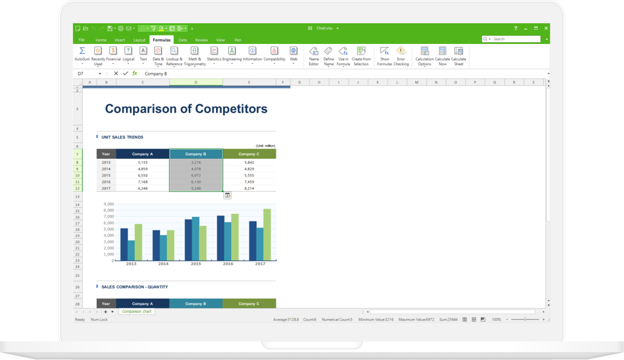
Microsoft Excel is a robust tool for data visualization and analysis. It usesspreadsheets to compile, organize, and analyze data with functions and formulas. 

Excel is popular among students, educators, marketers, accountants, data analysts, and other professionals. It is a component of the Microsoft Office suite. 

If you want alternatives to Microsoft Excel, you can check out our post on Top Excel alternatives, which include Truly Sheets, Google Sheets, Numbers and more.

Discover more alternatives to Excel here or see the best Dynamic Arrays alternatives.

What are Excel's uses?

Excel is adept at storing, analyzing, and presenting extensive data sets. It is commonly used by finance teams for financial analysis but is versatile enough for any professional handling large data sets. Excel uses range from creating financial statements and budgets to editorial schedules.

Excel is primarily used for crafting financial documents due to its potent calculation capabilities. It is often used within accounting departments because it offers automated insights into sums, averages, and totals, enabling accountants to interpret their business data efficiently.

While primarily known for its financial applications, Excel's functionality benefits all professionals, including marketers. It allows tracking of any data type without the hours spent manually counting or transferring data. Excel generally offers a shortcut or solution to expedite tasks.

After downloading the templates, let’s dive into using the software, starting with the basics.

Excel Fundamentals

If you're new to Excel, familiarize yourself with some essential commands, including:

• Creating a spreadsheet from scratch.
• Conducting basic arithmetic like addition, subtraction, multiplication, and division.
• Writing and formatting text and titles in columns.
• Utilizing Excel's auto-fill features.
• Adding or removing individual columns, rows, and spreadsheets. We will discuss adding multiple columns and rows later.
• Maintaining visibility of column and row headers as you scroll.
• Sorting your data alphabetically.

Let’s delve deeper into some of these fundamentals.

For instance, why is auto-fill significant?

If you know the basics of Excel, you're probably familiar with this quick feature. Nonetheless, let me demonstrate its utility. The auto-fill function lets you quickly populate adjacent cells with data, series, or formulas.

There are several methods to apply this feature, but the fill handle is one of the simplest. Select your source cells, find the fill handle at the lower-right corner, and drag it across the cells you want to fill or double-click it.Additionally, sorting is a crucial feature when organizing data in Excel.

Sometimes, your data list may be completely unsorted. For example, you might have exported a list of marketing contacts or blog entries. Whatever your scenario, Excel's sort function can alphabetize any list.

Click the column with the data you wish to sort, head to the “Data” tab on your toolbar, and locate the “Sort” option on the left. If “A” is above “Z,” click once to sort. If “Z” is above “A,” click twice. When “A” is on top, your list will sort alphabetically, and vice versa for reverse order.

Next, let’s further explore Excel's basics and more advanced features.

How to Operate Excel

To operate Excel, simply input data into the rows and columns, then use formulas and functions to transform that data into insights.

We’ll discuss essential formulas and functions shortly, but first, let’s review the types of documents you can generate using Excel. This will give you a comprehensive understanding of how Excel can be integrated into your daily tasks.

Documents You Can Create in Excel

Unsure how Excel can serve your team? Here’s a list of documents you can generate:

• Income Statements: An Excel spreadsheet tracks a company’s sales activity and financial health.
• Balance Sheets: Commonly created in Excel, these provide a comprehensive view of a company’s financial status.
• Calendars: Easily create a spreadsheet calendar to monitor events or other date-sensitive information.

Here are some documents specifically useful for marketers:

• Marketing Budgets: Excel is a powerful tool for budget management. Create and monitor marketing budgets and expenditures with Excel. For ready-made solutions, download our free marketing budget templates.
• Marketing Reports: Without a dedicated marketing tool like Marketing Hub, you might need a dashboard for all your reports. Excel is perfect for creating comprehensive marketing reports. Download free Excel marketing reporting templates here.
• Editorial Calendars: Excel's tab format simplifies tracking your content creation over custom time periods. Access a free editorial content calendar template here.
• Traffic and Leads Calculator: Excel's advanced calculation capabilities make it an ideal tool for developing calculators, including tracking leads and traffic. Download a free ready-to-use lead goal calculator here.

This list is just a glimpse of the numerous marketing and business documents you can create with Excel. We have compiled an extensive list of Excel templates immediately available for use in marketing, invoicing, project management, budgeting, and more.

In the interest of efficiency and eliminating tedious, manual tasks, here are several Excel formulas and functions you should know.

Excel Formulas

You might feel overwhelmed by the many formulas available if you're new to Excel. However, the following basic formulas can perform some complex functions without complicating your learning curve.

• Equal sign: Start any formula with an equal sign (=) in the cell where you want the result to appear.
• Addition: To sum the values in two or more cells, use the + sign. Example: =C5+D3.
• Subtraction: To subtract values from different cells, use the - sign. Example: =C5-D3.
• Multiplication: To multiply values from different cells, use the * sign. Example: =C5*D3.
• Division: To divide values from different cells, use the / sign. Example: =C5/D3.

You can combine these operations in a single cell. Example: =(C5-D3)/((A5+B6)*3).

For more intricate formulas, encase expressions in parentheses to manage the order of operations properly. Remember that you can include plain numbers in your formulas.

Excel Functions

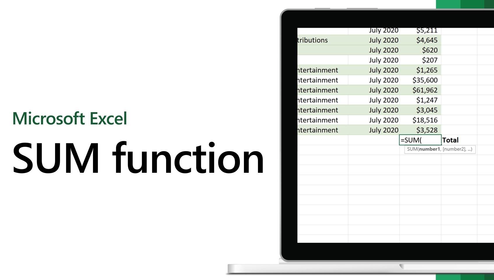
Excel functions automate tasks that you would typically handle via formulas. For example, instead of using the + sign to add up a range of cells, you'd use the SUM function. Here are a few more functions that can simplify calculations and tasks.

• SUM: This function automatically sums a range of cells or numbers. Specify the starting and ending cells with a colon between them. Example: =SUM(C5:C30).
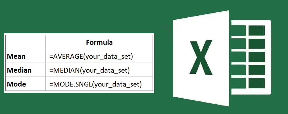
• AVERAGE: This function calculates the average of a range of cells. The syntax mirrors the SUM function: AVERAGE(Cell1:Cell2). Example: =AVERAGE(C5:C30).
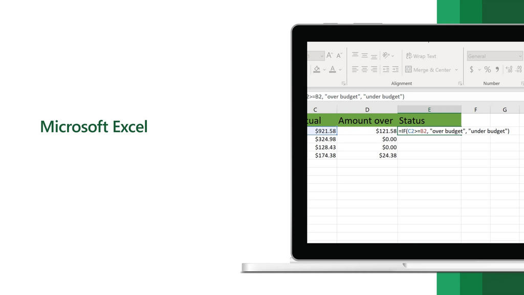
• IF: This function returns values based on a logical test. The syntax is as follows: IF(logical_test, value_if_true, [value_if_false]). Example: =IF(A2>B2,"Over Budget","OK").
• VLOOKUP: This function assists in searching for data across your sheet’s rows. The syntax includes: VLOOKUP(lookup value, table array, column number, Approximate match (TRUE) or Exact match (FALSE)). Example: =VLOOKUP([@Attorney],tbl_Attorneys,4,FALSE).
• INDEX: This function retrieves a value from within a range. The syntax is: INDEX(array, row_num, [column_num]).
• MATCH: This function locates a specific item in a range of cells and returns its position. It's often used together with the INDEX function. The syntax is: MATCH(lookup_value, lookup_array, [match_type]).
• COUNTIF: This function counts the number of cells that meet a specific criterion or contain a particular value. The syntax is: COUNTIF(range, criteria). Example: =COUNTIF(A2:A5,"London").

Excel Tips

1. Utilize Pivot tables to organize and interpret data.
2. Add multiple rows or columns simultaneously.
3. Simplify your datasets with filters.
4. Eliminate duplicate data entries or sets.
5. Convert rows to columns and vice versa.
6. Split text data across multiple columns.
7. Employ simple calculation formulas.
8. Calculate the average of numeric values in cells.
9. Apply conditional formatting for dynamic cell color changes based on data.
10. Automate tasks with the IF Excel formula.
11. Lock a cell's formula with dollar signs to prevent changes during movement.
12. Retrieve data across sheets with the VLOOKUP function.
13. Pull data from horizontal columns with INDEX and MATCH formulas.
14. Count words or numbers in any cell range with the COUNTIF function.
15. Concatenate cells using the ampersand symbol.
16. Incorporate checkboxes for interactive data tracking.
17. Link cells to websites with hyperlinks.
18. Add drop-down menus for streamlined data entry.
19. Copy formatting quickly with the format painter.
20. Create and manage data with tables.
21. Perform what-if analyses to simulate different scenarios.
22. Name ranges for easier formula management.
23. Organize your data with grouping.
24. Use Find & Select for efficient formatting.
25. Safeguard your work with protection features.
26. Design custom number formats for unique data presentation.
27. Customize the Excel ribbon for optimized workflow.
28. Enhance readability with text wrapping.
29. Incorporate emojis for a personalized touch.

Note: Updates have been made to accommodate users of both new and older versions.

Use Pivot tables to understand and organize data

Pivot tables are excellent for reorganizing spreadsheet data. They don't alter your data but can summarize and compare different information based on your needs.

To create a Pivot Table, go to Data > Pivot Table. In the latest version of Excel, you’d go to Insert > Pivot Table. Excel automatically sets up your Pivot Table, but you can modify the data arrangement. Then, choose from four options:

• Report Filter: This lets you view only specific rows in your dataset. For instance, you might include only Gryffindor students to filter by house.
• Column Labels: These serve as your dataset headers.
• Row Labels: These could be your dataset rows. Row and Column labels can include data from your columns (e.g., First Name could be placed in either Row or Column labels depending on your data viewing preference).
• Value: This section allows you to view your data differently. Instead of pulling any numeric value, you can sum, count, average, or perform other manipulations. By default, dragging a field to Value usually counts it.

Add multiple rows or columns

You might often need to insert additional rows or columns as you work with your data. Sometimes, you may need to add hundreds at once. Adding them one by one would be laborious. Fortunately, there’s a simpler way.

To add multiple rows or columns in a spreadsheet, highlight the same number of existing rows or columns you want to add. Right-click and select “Insert.”

In the example below, I need to add three more rows. By selecting three existing rows and clicking insert, I can quickly include three new blank rows in my spreadsheet.

Apply filters to streamline your data

You don’t need to view every row simultaneously when working with large datasets. Sometimes, you only need to see data that meet specific criteria.

That’s where filters come into play.

Filters allow you to narrow down your data to view only certain rows at a time. In Excel, you can add a filter to each column in your dataset. From there, you can select which cells you wish to see simultaneously.

Let’s consider the following example. Add a filter by selecting the Data tab and clicking "Filter." Clicking the arrow next to column headers lets you choose how you want your data organized—in ascending or descending order—and which specific rows to display.

Pro Tip: To further analyze your data, copy and paste the values in the spreadsheet while a Filter is active into a separate spreadsheet.

Remove duplicate data points or sets

Large datasets often contain duplicate information. For example, you might have multiple contacts from the same company and only want to view unique companies. In such cases, removing duplicates is extremely useful.

To eliminate duplicates, highlight the row or column where duplicates are present. Then, go to the Data tab and select “Remove Duplicates” (located under the Tools subheader in older versions of Excel). A pop-up will confirm which data you want to process. Select “Remove Duplicates,” and you’re set.

You can also use this feature to eliminate an entire row based on duplicate column values. So, if you have multiple entries for Harry Potter and only need one, select the entire dataset and remove duplicates based on email. Your list will then only show unique names without duplicates.

Convert rows into columns

If you have rows of data and decide you want to convert them into columns (or vice versa), copying and pasting each header would be time-consuming. However, the transpose feature simplifies this process.

Start by selecting the column you want to turn into rows. Right-click it, and choose “Copy.” Next, select the cells where you want your first row or column to start. Right-click on the cell, and select “Paste Special.” A module will appear—at the bottom, you'll see an option to transpose. Check that box and select OK. Your column will now be transferred to a row, or vice versa.

In newer versions of Excel, a drop-down will appear instead of a pop-up.

Excel transpose tool in newer versions

Divide text information between columns

What if you need to split information in one cell into two different cells? For example, you might want to extract a company name from an email address or separate a full name into first and last names for your email marketing templates.

Thanks to Excel, both tasks are achievable. First, highlight the column you want to split. Next, go to the Data tab and select “Text to Columns.” A module with additional options will appear.

First, decide whether you want “Delimited” or “Fixed Width.”

• “Delimited” means breaking up the column based on characters like commas, spaces, or tabs.
• “Fixed Width” means choosing the exact location across the columns where you want the split to occur.

Choose “Delimited” to separate the full name into first and last names.

Then, select your Delimiters. This could be a tab, semi-colon, comma, space, or something else. ("Something else" could be the "@" sign used in an email address, for example.) In our example, let’s choose the space. Excel will then show you how your new columns will look.

When you’re satisfied with the preview, press "Next." This page will let you select Advanced Formats if desired. When you’re ready, click “Finish.”

Use simple calculation formulas

Excel can handle both complex and simple calculations. Here’s how to perform basic arithmetic:

• To add, use the + sign.
• To subtract, use the - sign.
• To multiply, use the * sign.
• To divide, use the / sign.

You can also use parentheses to ensure certain calculations are prioritized. In the example below (10+10*10), the second and third 10s are multiplied before adding the first 10. However, if it were (10+10)*10, the first two 10s would be added first.

Calculate the average of numbers in your cells.

To find the average of a set of numbers, use the formula =AVERAGE(Cell1:Cell2). To sum a column of numbers, use the formula =SUM(Cell1:Cell2).

Apply conditional formatting for dynamic cell coloring

Conditional formatting lets you change a cell's color based on the data within. For instance, you can highlight numbers that are above average or in the top 10% of your data. This feature is also useful for visually linking commonalities between different rows in Excel. It enables you to identify important information quickly.

To begin, select the group of cells for conditional formatting. Then, choose “Conditional Formatting” from the Home menu and pick your logic from the dropdown. (You can also create a custom rule if needed.) A window will appear, prompting you to detail your formatting rule. Click “OK” when finished, and your results will automatically display.

Automate tasks with the IF Excel formula

Sometimes, you don't just want to count the number of times a value appears; you want to input different information into a cell based on another cell's data.

The formula is: IF(logical_test, value_if_true, [value_if_false])

Generally, the formula structure is IF(Logical Test, value if true, value if false). Let’s explore these components.

• Logical_Test: This is the condition for the “IF” part of the formula. In this example, the condition is D2="n" because we want to ensure the cell corresponding with the student reads “n.” Make sure to use quotation marks around n.
• Value_if_True: The cell should display this if the condition is true. Here, we want “10” to indicate the student was awarded the points. Use quotation marks if the result is text.
• Value_if_False: The cell should display this if the condition is false. Here, for any student not in Gryffindor, we want “0”. Use quotation marks if the result is text.

The real strength of the IF function emerges when you nest multiple IF statements together, allowing you to set multiple conditions, get more specific results, and better organize your data.

Ranges are another way to segment your data for analysis. For instance, you can categorize data into values less than 10, 11 to 50, or 51 to 100. Here’s what that looks like in practice:

=IF(B3<11,"10 or less",IF(B3<51,"11 to 50",IF(B3<100,"51 to 100")))

It may require some trial and error, but once you master it, IF formulas will become your new best friend in Excel.

Lock cell formulas with dollar signs.

Have you noticed dollar signs in an Excel formula? These aren’t represent American dollars; instead, they ensure that the specific column and row remain constant, even if you copy the formula to adjacent rows.

Normally, a cell reference—like referring to cell A5 from cell C5—is relative by default. In this case, you’re referring to a cell five columns to the left (C minus A) and in the same row (5). 

This is known as a relative formula. Copying a relative formula from one cell to another adjusts the formula values based on its new location. But sometimes, you want those values to remain unchanged, regardless of their position—and you can achieve this by converting the formula to an absolute formula.

To transform a relative formula (=A5+C5) into an absolute formula, precede the row and column values with dollar signs, like this: (=$A$5+$C$5). (Learn more on Microsoft Office's support page here.)

Retrieve data across sheets with the VLOOKUP function.

Ever had two different sets of data on separate spreadsheets that you wanted to merge into one?

For instance, you might have a list of people’s names next to their email addresses on one sheet, and a list of those same people’s email addresses next to their company names on another—but you want the names, email addresses, and company names to appear together.

I often need to combine datasets like this—and when I do, VLOOKUP is my go-to formula.

Before using the formula, ensure you have at least one column that appears identically in both datasets. Check your data to ensure the column you’re using to merge your information is exactly the same, including no extra spaces.

The formula: =VLOOKUP(lookup value, table array, column number, Approximate match (TRUE) or Exact match (FALSE))

The formula with variables from our example below: =VLOOKUP(C2,Sheet2!A:B,2,FALSE)

In this formula, several variables are involved. Here’s what’s true when you want to combine information from Sheet 1 and Sheet 2 onto Sheet 1:

• Lookup Value: This is the identical value present in both spreadsheets. Select the first value in your first spreadsheet. In the example, this means the first email address on the list, or cell C2.
• Table Array: The table array is the range of columns on Sheet 2 you’re pulling data from, including the column of data identical to your lookup value (in our example, email addresses) in Sheet 1 as well as the column of data you’re copying to Sheet 1. In our example, this is “Sheet2!A:B.” “A” means Column A in Sheet 2, which contains the data identical to our lookup value (email) in Sheet 1. The “B” means Column B, which has the information only available in Sheet 2 that we want to transfer to Sheet 1.
• Column Number: This specifies which column in Sheet 2 contains the new data you want to copy to Sheet 1. In our example, this would be the column where “House” is located. “House” is the second column in our range (table array), so our column number is 2. [Note: Your range can include more than two columns. For example, if there are three columns on Sheet 2—Email, Age, and House—and you still want to bring “House” onto Sheet 1, you can still use a VLOOKUP. You just need to change the “2” to a “3” so it pulls back the value in the third column: =VLOOKUP(C2:Sheet2!A:C,3,false).]
• Approximate Match (TRUE) or Exact Match (FALSE): Use FALSE to ensure only exact value matches are pulled. If you use TRUE, the function will pull approximate matches.

So when we input the formula =VLOOKUP(C2,Sheet2!A:B,2,FALSE), we bring all the house data into Sheet 1.

Keep in mind that VLOOKUP will only pull back values from the second sheet that are to the right of the column containing your identical data. This can be limiting, which is why some people prefer using the INDEX and MATCH functions instead.

Retrieve data from horizontal columns with INDEX and MATCH formulas.

Like VLOOKUP, the INDEX and MATCH functions pull data from another dataset into a central location. Here are the main differences:

• VLOOKUP is simpler. However, if you’re dealing with large data sets that require thousands of lookups, using INDEX and MATCH will significantly decrease Excel’s load time.
• INDEX and MATCH work right-to-left, whereas VLOOKUP only works left-to-right. If your lookup column is to the right of the results column, you’d need to rearrange those columns to use VLOOKUP, which can be tedious with large datasets and potentially lead to errors.

If I want to combine information from Sheet 1 and Sheet 2 onto Sheet 1, but the column values in Sheets 1 and 2 aren’t the same, then I’d use INDEX and MATCH instead of VLOOKUP to avoid rearranging my columns.

Let’s explore an example. Let’s say Sheet 1 contains a list of people’s names and their Hogwarts email addresses, and Sheet 2 contains a list of people’s email addresses and the Patronus associated with each student. 

The email address column is in different column numbers on each sheet. I’d use the INDEX and MATCH formulas instead of VLOOKUP so I wouldn’t have to switch any columns around.

So, what’s the formula? It’s actually the MATCH formula nested inside the INDEX formula. You’ll notice I differentiated the MATCH formula using a different color here.

The formula: =INDEX(table array, MATCH formula)

This becomes: =INDEX(table array, MATCH(lookup_value, lookup_array))

The formula with variables from our example below: =INDEX(Sheet2!A:A,(MATCH(Sheet1!C:C,Sheet2!C:C,0)))

Here are the variables:

• Table Array: The range of columns on Sheet 2 containing the new data you want to bring to Sheet 1. In our example, “A” means Column A, which contains each person's “n” information.
• Lookup Value: This column in Sheet 1 contains identical values in both spreadsheets. The example refers to the “email” column on Sheet 1, which is Column C. So: Sheet1!C:C.
• Lookup Array: This column in Sheet 2 contains identical values in both spreadsheets. In the example, this refers to the “email” column on Sheet 2, which also happens to be Column C. So: Sheet2!C:C.

Once you have sorted your variables, type the INDEX and MATCH formulas into the top cell of the blank Patronus column on Sheet 1, where you want the combined information to reside.

Count words or numbers in any range of cells with the COUNTIF function.

Rather than manually counting how often a specific value or number appears, let Excel handle it. With the COUNTIF function, Excel can count how many times a word or number shows up in any range of cells.

For instance, let's say I want to count the number of times the word “n” appears in my data set.

The formula: =COUNTIF(range, criteria)

The formula with variables from our example below: =COUNTIF(D:D,"n")

In this formula, there are several variables:

Range: The range you want the formula to cover. In this case, since we’re focusing on one column, we use “D:D” to indicate that both the first and last column are D. If I were examining columns C and D, I would use “C:D.”

Criteria: The number or piece of text you want Excel to count. Use quotation marks if you want the result to be text, not a number. In our example, the criteria is “n.”

Simply entering the COUNTIF formula into any cell and pressing “Enter” will display how many times the word “n” appears in the dataset.

Concatenate cells using &.

Databases often separate data to make it as precise as possible. For example, instead of having a column that shows a person’s full name, a database might separate it into first and last names in different columns. Or, it might divide a person’s location by city, state, and zip code. In Excel, you can combine cells with different data into one cell using your function's “&” sign.

The formula with variables from our example below: =A2&" "&B2

Let’s walk through the formula together using an example. Suppose we combine first and last names into full names in a single column. We’d first place our cursor in the blank cell where we want the full name to appear. Next, we'd highlight a cell containing a first name, type in an “&” sign, and then highlight a cell with the corresponding last name.

But you’re not done—if all you type in is =A2&B2, there will be no space between the person’s first and last names. To add the necessary space, use the function =A2&" "&B2. The quotation marks around the space instruct Excel to insert a space between the first and last names.

To apply this to multiple rows, drag the corner of that first cell downward, as shown in the example.

Add checkboxes.

If you’re using an Excel sheet to track customer data and need to monitor something non-quantifiable, you could insert checkboxes into a column.

For example, if you’re managing sales prospects in an Excel sheet and want to track whether you contacted them in the last quarter, you could have a "Called this quarter?" column and check off the cells when you’ve contacted the respective client.

Here’s how to do it.

Highlight the cell where you’d like to add checkboxes in your spreadsheet. Then, click DEVELOPER. Under FORM CONTROLS, click the checkbox or the selection circle in the image below.

Once the box appears in the cell, copy it, highlight the cells where you want it to appear, and then paste it.

Link cells to websites with hyperlinks

If you’re using your sheet to track social media or website metrics, having a reference column with links for each row can be helpful. If you add a URL directly into Excel, it should automatically become clickable. However, if you need to hyperlink words like a page title or the headline of a post you’re tracking, here’s how.

Highlight the words you want to hyperlink, then press Shift K. A box will pop up allowing you to enter the hyperlink URL. Copy and paste the URL into this box and hit or click Enter.

If the key shortcut isn't working for any reason, you can do this manually by highlighting the cell and clicking Insert > Hyperlink.

Add drop-down menus.

Sometimes, you’ll use your spreadsheet to track processes or other qualitative data. Rather than repeatedly typing words into your sheet, such as "Yes", "No", "Customer Stage", "Sales Lead", or "Prospect", you can use dropdown menus for quick, consistent data entry.

Here’s how to add drop-downs to your cells.

Highlight the cells where you want the drop-downs, then click the Data menu in the top navigation and press Validation.

From there, a Data Validation Settings box will open. Look at the Allow options, then click Lists and select Drop-down List. Check the In-Cell dropdown button, then press OK.

Copy formatting quickly with the format painter

As you’ve probably noticed, Excel offers many features to expedite number crunching and data analysis. However, if you’ve spent time formatting a sheet to your liking, you know it can become tedious.

Don’t waste time repeating the same formatting commands. Use the format painter to easily copy formatting from one worksheet area to another. To do so, choose the cell whose formatting you’d like to replicate, then select the format painter option (paintbrush icon) from the top toolbar.

Create and manage data with tables

Converting your data into a table makes it visually appealing and enhances data management and analysis capabilities.

To begin, select the range of cells you want to convert into a table. Then, go to the Home tab in the Excel ribbon. In the Styles group, click on the Format as Table button—it looks like a grid of cells. Choose a table style from the available options, or customize a table if desired.

In the Create Table dialog box, ensure the selected range is correct. If Excel did not automatically detect the range accurately, you can adjust it manually. If your table includes headers (column names), check the “My table has headers” option. This allows Excel to treat the first row as the header row.

Once everything is set, click the OK button, and Excel will convert your selected data into a table.

After your data is converted into a table, you’ll notice some additional features and functionalities become available:

• The table is automatically assigned a name, such as “Table1” or “
• Filter drop-down arrows appear in the header row, allowing you to filter data within the table easily.
• The table is formatted with alternating row colors, making it visually appealing.
• Total rows are automatically added at the bottom of each column, allowing you to perform calculations like sum, average, etc., for the data in that column.

Use tables to conduct what-if analyses.

In addition to making your data more organized, tables can help you conduct what-if analyses. This allows you to test various combinations of input values and observe the resulting outcomes.

A what-if analysis can be beneficial in decision-making, planning, forecasting, financial modeling, sensitivity analysis, resource planning, and more.

You’ll need to set up your worksheet with the necessary formulas and variables you want to analyze to get started. Then, determine the input values that you want to vary. Typically, you will choose one or two input variables.

Select the cell where you want to display the results of your what-if analysis. Then, click the What-If Analysis button to the Data tab in the Excel ribbon. From the dropdown menu, select Data Table.

In the Table Input dialog box, enter the input values you want to test for each variable. Enter the input values in a column or row if you have one variable. If you have two variables, enter the combinations in a table format.

Select the cells in the table area corresponding to the formula cell you want to analyze. This cell will display the results for each combination of input values.

Click OK to generate the data table. Excel will calculate the formula for each combination of input values and display the results in the selected cells. The data table acts as a grid, showing the various scenarios and their corresponding outcomes.

Once your table is created, you can use it to identify trends, patterns, or specific values of interest. Play around with the input values and see how it may affect the final results.

Make formulas easier to comprehend with named ranges.

Instead of referring to a range of cells by its coordinates (e.g., A1:B10), you can assign a name. This makes formulas more readable and easier to manage.

To get started, select the cell or range you want to name. Go to the Formulas tab in the Excel ribbon and click the Define Name button in the Defined Names group. Alternatively, you can use the keyboard shortcut Alt + M + N + D.

In the New Name dialog box, enter a name for the selected cell or range in the Name field. Make sure the name is descriptive and easy to remember. By default, Excel assigns the selected cell or range's reference to the Refers to field in the dialog box. You can modify the reference to include additional cells or adjust the range if needed.

Click the OK button to save the named range. Once you've named a range, you can use it in your formulas by simply typing the name instead of the cell reference. For example, if you named cell A1 as “Revenue,” you could use =Revenue instead of =A1 in your formulas.

Using named ranges offers several benefits:

• Improved formula readability: Named ranges make formulas easier to understand and navigate, especially in complex calculations or large datasets.
• Flexibility for range adjustments: If your dataset changes, you can easily modify the range assigned to a named range without updating each formula that references it.
• Enhanced collaboration: Named ranges make it easier to collaborate with others, as they can understand the purpose of a named range and use it in their own calculations.
• Simplified data analysis: When using named ranges, you can create more intuitive data analysis by referring to named ranges in functions like SUM, AVERAGE, COUNTIF, etc.

To manage named ranges, you can go to the Formulas tab, click on the Name Manager button in the Defined Names group. The Name Manager offers functionalities to modify, delete, or review existing named ranges.

Organize your data with grouping

Grouping data in Excel allows you to organize, analyze, and present information more effectively, making it easier to identify patterns, trends, and insights within your data. For instance, if you have a list of leads generated, you can group the data by month to create a monthly performance report.

Grouping data makes navigating and working with large data sets easier. It helps in organization and reduces clutter by collapsing the groups that are not immediately needed.

To group data in Excel, select the range of cells or columns you want to group. If necessary, sort the data properly.

Click on the Group button on the Data tab in the Excel ribbon. It is usually found in the Outline or Data Tools group.

You can specify the grouping levels by choosing options like Rows or Columns. For example, you can select Months if you want to group data by month. You can also set additional options such as Summary rows below detail or Collapse the outline to the summary levels. These options affect how the grouped data is displayed.

Once you have selected the options, click on the OK button, and Excel will group the selected data based on your settings.

After your data is grouped, you will see a plus (+) or minus (-) button next to the grouped rows or columns. Clicking on the plus button expands the group to show the individual records, and clicking on the minus button collapses the group to hide the details.

Streamline formatting with Find & Select

Why format and clean up your spreadsheet manually when you can do it in just a few clicks? Using the Find & Select tool can help you maintain document accuracy and consistency.

To start, open the Excel worksheet containing the data you want to search. Press the Ctrl + F keys on your keyboard or go to the Home tab and click the Find & Select drop-down menu. Then, select Find from the menu. The Find and Replace dialog box will open.

In the Find field, enter the specific data you want to find. Then, you can choose the appropriate options in the dialog box to narrow down your search to specific cells, rows, columns, or formulas.

Click on the Find Next button to search for the first occurrence of the data. Excel will highlight the cell containing the data.

To replace the found data with new information, click the Replace button in the dialog box. This will replace the highlighted occurrence with the data you enter in the Replace field.

To replace all occurrences of the data at once, click on the Replace All button. You can close the dialog box once you have finished finding and replacing it.

Note: Be cautious when using the Replace All feature, as it replaces all occurrences without confirmation. Review each replacement carefully before using the Replace All option is always a good practice.

Protect your work

Protecting your work in Excel is essential for data security, maintaining data integrity, preserving intellectual property, and complying with legal or regulatory requirements. It allows you to control who can access and modify your work, minimizing risks and maintaining the quality and confidentiality of your data.

Here are a couple ways you can protect your work:

Protect a Worksheet

• Open your Excel worksheet and navigate to the Review tab.
• Click on the Manage Protection button in the Protection group.
• A Manage Protection dialog box will appear. There, you can select whether or not you want to protect the sheet. Set a password if desired and choose the options you want to apply, such as preventing users from making cell changes, formatting, inserting/deleting columns or rows, etc.

Protecting a Workbook

1. Open your Excel workbook and navigate to the File tab.
2. Click on Info and select Protect Workbook from the options.
3. Choose Encrypt with Password and enter a password if desired.
4. Click OK to protect the workbook.

Taking these extra steps ensures your work is protected. Just make sure to keep your passwords safe and secure.

26. Create custom number formats.

To display data in unique ways, use custom number formats. Doing this can help with data presentation, clarity, consistency, localization, and masking sensitive data.

To get started, select the cell or range you want to format. Right-click on the selected cells and choose Number Format from the context menu. Then, find the Category list and select Custom.

In the Type field, you can enter a custom number format code to define your desired format. Here are some examples of custom number formats:

To display numbers with a specific number of decimal places, use the 0 or # symbol to represent a digit, and a zero or hashtag without a decimal point to represent optional digits. For example, 0.00 will display two decimal places, 0.### will display up to three decimal places, and ### will display no decimal places.

To display a specific text or character alongside numbers, use the @ symbol. For example, $0 will display a dollar sign before the number.

To display percentages, use the % symbol. For example, 0% will display the number as a percentage.

To create custom date or time formats, use codes such as dd for day, mm for month, yy for two-digit year, hh for hours, mm for minutes, and ss for seconds. For example, dd/mm/yyyy will display the date in the format of day/month/year.

As you enter your custom number format in the Type field, you will see a Sample section showing how the format will be applied. Click OK to apply the custom number format to the selected cells.

27. Customize the Excel ribbon.

Although the Excel ribbon already contains various tools used to execute common functions and commands, you can customize it to fit your specific needs and preferences.

This can help streamline your workflow and make commonly used commands more easily accessible. It also allows you to remove unnecessary elements you don’t use, making navigating and finding the tools you need easier.

To make customizations, start by right-clicking on an empty area of the ribbon and selecting Customize the Ribbon. In the Excel Options window that appears, you'll see two sections. The left section displays the tabs currently visible in the ribbon, while the right section displays the tabs you can add.

To customize the ribbon, you have several options:

• To add a new tab, click on New Tab in the right section and give it a name.
• To add a group within an existing tab, select the tab in the left section, click New Group in the right section, and name it.
• To add commands to a group, select the group in the right section, choose commands from the left section, and click Add. You can also customize the order of the commands using the Up and Down buttons.

You can also remove tabs, groups, or commands from the ribbon. In the left section, select the item you want to remove and click Remove.

To change the order of tabs and groups, select the item in the left section and use the Up and Down buttons to rearrange them.

Click OK in the Excel Options window to save your changes and apply the customized ribbon.

To enhance Excel's capabilities further, you can personalize the ribbon by adding more apps through the 'Add-ins' button on the Home tab.

Note that customizing the ribbon only affects your personal Excel setup and does not impact the ribbons of other users.

28. Enhance the visual appeal with text wrapping.

Although spreadsheets may not be visually exciting, wrapping text can make them more readable by allowing multiple lines of text within a single cell. This is particularly useful for adding line breaks or dividing lengthy text into paragraphs within a cell without enlarging the row height.

To wrap text, select the cell(s) containing the text. Go to the top toolbar in Excel, find the 'Wrap Text' button (marked by an icon with an angled arrow) in the Alignment section, and click it.

29. Incorporate emojis

To insert an emoji, click on the cell, then activate the emoji keyboard, which varies by operating system:

• Windows: Use the shortcut Win + . or Win + ;
• macOS: Use Ctrl + Cmd + Space.

Browse and select your desired emoji to have it displayed in the cell.

Emojis may initially appear small in Excel cells. You can increase their size by adjusting the row height and column width. Alternatively, you can copy and paste emojis from the Internet or other applications directly into Excel cells.

Note: The ability to use emojis in Excel varies with the software version and device. Some older versions or systems might not support or display emojis correctly, so compatibility checks are important.

Excel Keyboard Shortcuts:

• Create a new workbook: PC: Ctrl-N | Mac: Command-N
• Select an entire row: PC: Shift-Space | Mac: Shift-Space
• Select an entire column: PC: Ctrl-Space | Mac: Control-Space
• Select the rest of a column: PC: Ctrl-Shift-Down/Up | Mac: Command-Shift-Down/Up
• Select the rest of a row: PC: Ctrl-Shift-Right/Left | Mac: Command-Shift-Right/Left
• Add a hyperlink: PC: Ctrl-K | Mac: Command-K
• Open the Format Cells window: PC: Ctrl-1 | Mac: Command-1
• Autosum selected cells: PC: Alt-= | Mac: Command-Shift-T

Final Thoughts

Excel often feels like a magical tool, effortlessly automating tasks with just a formula. Whether merging sheets, performing calculations, or consolidating data, Excel simplifies complex tasks, making it indispensable for finance professionals and beyond. 

Now that you're equipped with these top tips, tricks, and shortcuts, you can elevate your Excel skills immediately, even without expert-level knowledge. Dive into these features to streamline tasks, enhance data presentations, and ensure efficiency. 

Ready to transform your spreadsheets? Start implementing these strategies today and witness a significant boost in your productivity.

Keep Learning

» Excel Tutorial for Beginners: Tips You Need to Know
» 13 Tips To Master Excel Without Breaking a Sweat
» Essential Excel Skills for All Levels
» 14 Excel Tricks That Will Impress Your Boss
» 13 Excel Tips and Tricks to Make You Into a Pro

Even with advanced formulas, every formula requires its own cell. However, this has changed drastically with the introduction of dynamic arrays in Excel, allowing a single formula to populate multiple cells. 

Microsoft’s upgrade to Excel’s calculation engine made this revolutionary feature possible.

The term "dynamic arrays" might initially seem complex, but its simplicity and power become evident once you understand how it works. The ability to fill multiple cells with a single formula marks a fundamental shift in how Excel operates.

Note: At the time of writing, dynamic arrays are only available in Excel 365, Excel Online, and Excel 2021. Older versions like Excel 2019 and earlier will not receive this feature.

Overview of Dynamic Arrays

Let’s start with a simple example to illustrate the impact of dynamic arrays:

=B2:B6

This formula might seem unusual, but it effectively demonstrates how dynamic arrays work. Previously, Excel could only return one result per formula. 

Now, a single formula can automatically return multiple results, spilling them into adjacent cells.

Before Dynamic Arrays

In Excel 2019 and earlier, a formula could only return one cell result. If a formula attempted to return multiple results, Excel made assumptions about which data to return, often leading to varying outcomes.

• If the formula aligned with the data, Excel assumed you wanted the value from the same row.
• If the formula was not in line, Excel returned a #VALUE! error.

In the image above:

• Cell D2 shows the value from B2 since it aligns with the source data.
• Cell D4 returns the value from B4 for the same reason.
• Cell D7, which does not align with the data, returns a #VALUE! error.

This behavior, known as implicit intersection, has been eliminated with dynamic arrays.

With Dynamic Arrays

In newer Excel versions that support dynamic arrays, the formula returns all five values, automatically populating multiple cells.

The terminology:

• Spilling: The action of filling multiple cells with a single formula.
• Spill Range: The range of cells filled by the formula.

Dynamic arrays enable a single formula to populate multiple cells, effectively eliminating the need for repetitive formulas in adjacent cells. Instead of copying formulas down manually, the entire result set can be obtained with a single command.

Which Versions of Excel Have Dynamic Arrays?

Dynamic arrays were introduced in September 2018 for early testers who signed up to receive previews of new Excel features. Over time, Microsoft gradually rolled out this feature to all Excel 365 users:

• Monthly Channel: From November 2019.
• Semi-Annual Channel: From July 2020.

Excel 2019 and earlier versions won’t be updated to include this feature. To access dynamic arrays, you need Excel 2021 or Microsoft 365. The dynamic array feature is exclusive to the latest versions, so it’s worth upgrading if you work with Excel frequently.

New Dynamic Array Functions

Alongside dynamic arrays, Microsoft introduced six new functions that leverage this powerful feature:

1. UNIQUE: Lists unique or distinct values in a range.
2. SORT: Sorts values in a range.
3. SORTBY: Sorts values based on another column.
4. FILTER: Returns only values meeting specific criteria.
5. SEQUENCE: Generates a sequence of numbers.
6. RANDARRAY: Returns an array of random numbers.

These new functions help illustrate the versatility of dynamic arrays. The real game-changer, however, is that dynamic arrays affect not only these new functions but also how Excel handles all formulas.

UNIQUE

The UNIQUE function identifies unique values in a range. For instance, consider the following formula:

=UNIQUE(A2:A10)

This formula returns only the distinct values from the specified range. Dynamic arrays enable the results to spill across multiple cells automatically.

SORT

The SORT function organizes data in ascending or descending order. Here’s an example:

=SORT(A2:A10, 1, 1)

The second argument specifies the column to sort by (1 means the first column), and the third argument indicates the sort order (1 for ascending and -1 for descending).

SORTBY

The SORTBY function sorts values based on another column or range:

=SORTBY(A2:A10, B2:B10, 1)

This sorts the range A2:A10 based on the corresponding values in the B2:B10 range.

FILTER

The FILTER function returns only values meeting specific criteria:

=FILTER(A2:A10, B2:B10="Completed")

This formula retrieves all values in A2:A10 where the corresponding value in B2:B10 equals "Completed."

SEQUENCE

The SEQUENCE function generates a sequence of numbers:

=SEQUENCE(5, 1)

This formula returns a column with five rows of consecutive numbers. The first argument specifies the number of rows, and the second argument indicates the number of columns.

RANDARRAY

The RANDARRAY function returns an array of random numbers:

=RANDARRAY(5, 2)

This formula generates a 5-row by 2-column array of random values.

Dynamic Array Formulas

Apart from the new functions, many existing functions like SUMIFS and VLOOKUP can now spill.

Before Dynamic Arrays

To calculate the total score for each person, we used to apply SUMIFS like this:

=SUMIFS($C$2:$C$9,$B$2:$B$9,E2)

This formula would then be copied down for each individual:

With Dynamic Arrays

With dynamic arrays, one formula can achieve the same result:

=SUMIFS(C2:C9,B2:B9,E2:E5)

The formula returns all results, spilling them into cells F2-F5.

The power of dynamic arrays lies in the ability to adjust to changes in data ranges automatically. When new rows are added to the data, the spill range expands or contracts accordingly, making it incredibly efficient and reducing the need for manual adjustments.

Which Formulas Spill?

Functions like SUM, AVERAGE, MIN, and MAX won’t spill themselves since they expect a range of values and only return one result.

However, functions like VLOOKUP spill when given multiple scalars (individual values). For example, VLOOKUP in cell F7 looks up "Dave" and "Jack," returning their scores across multiple rows.

In the example above, the formula is:

=VLOOKUP(E7:E8, B2:D5, 2, FALSE)

This retrieves scores for both "Dave" and "Jack" from the range B2:D5. Dynamic arrays handle the calculations instead of writing multiple formulas in one go.

Other Functions

Generally, any function with an argument that expects a single value (a scalar) is likely to spill if given multiple values instead.

• INDEX: Returns multiple values if the row or column argument is a range.
• IF: Can spill results if the logical test returns multiple values.
• MATCH: Returns multiple matches if given an array.

The new calculation engine fundamentally changes how Excel formulas operate, enabling users to work more efficiently with their data.

Spilling

When a formula spills, a blue outline appears around the spill range, indicating the area filled by the formula. Editing can only occur from the top-left cell. Other cells in the spill range will display a grayed-out formula version.

If data is blocking the spill range, Excel returns a #SPILL! error. Clicking on the error shows the spill range and indicates what’s causing the problem.

Common Reasons for #SPILL! Errors

1. Spill Range Exceeds Worksheet Boundaries: The spill range extends beyond the available rows and columns of the worksheet.
2. Unknown Spill Range Size: Excel cannot determine the size of the spill range.
3. Dynamic Array Formula Placed Inside a Table: Excel tables do not support dynamic array formulas.
4. Spill Range Contains Merged Cells: Merged cells can prevent results from spilling.
5. Excel Runs Out of Memory: The spill range is too large for Excel to handle.

Resolving #SPILL! Errors

To resolve these errors, ensure that:

• The spill range fits within the worksheet.
• No data blocks the spill range.
• Dynamic array formulas are not placed inside tables.
• There are no merged cells in the spill range.

# References

Use the # symbol to refer to the entire spill range. For example, if the top-left cell is F2, then F2# will reference all cells in the spill range.

The formula =AVERAGE(F2#), and the # symbol ensures the average covers all spilled values.

Advantages of # References

1. Automatic Expansion: The reference expands or contracts as the spill range changes.
2. Flexibility: Makes working with dynamic data simpler and more intuitive.
3. Less Maintenance: Reduces the need for manual adjustments to formulas.

Example with # References

The # reference dynamically includes all values in the spill range F2# in the following formula.

=SUM(F2#)

This ensures the total sum always includes the full range, even if the number of rows changes.

Constant Arrays

Constant arrays have existed in Excel for some time, but dynamic arrays have made their usage more popular. Here's an example with VLOOKUP:

=VLOOKUP(F6,B2:D5,{2,3},0)

This formula returns values (2 and 3) in columns G3 and H3. Commas separate columns, while semicolons separate rows.

To spill results across rows instead of columns, use semicolons:

=VLOOKUP(F6,B2:D5,{2;3},0)

Creating Constant Arrays

Constant arrays can be created manually by enclosing the desired values in curly braces {}.

• Columns: Separate values with commas {1,2,3}
• Rows: Separate values with semicolons {1;2;3}

Examples

1. Horizontal Array: {1, 2, 3}
2. Vertical Array: {1; 2; 3}
3. 2D Array: {1, 2; 3, 4}

Application with Functions

Constant arrays can be used with various functions to produce dynamic results. For example:

=SUM({1,2,3})

This sums up the values within the constant array.

=VLOOKUP(F6,B2:D5,{2,3},0)

This retrieves values from multiple columns simultaneously using a constant array.

The @ Symbol

The @ symbol forces Excel to operate in the old implicit intersection mode. Let’s revisit our original example:

=B2:B6

Add the @ symbol to use the old implicit intersection method, which only returns values in the same row.

=@B2:B6

Backward Compatibility:
To ensure backward compatibility, the @ symbol is added automatically to some formulas. This ensures that workbooks created in older versions of Excel continue to calculate the same results when opened in the newer version.

Structured References and the @ Symbol

The @ symbol is also used in structured references with Excel tables to reference items in the same row.

=[@Column1]

This refers to the value in "Column1" within the table's current row.

Examples of @ Usage

1. Single Value Lookup: =@VLOOKUP(E2,B2:C10,2,FALSE)
2. Table References: =SUM([@Sales])

Summary of @ Symbol Usage:

• Backward Compatibility: Automatically added to formulas from older Excel versions.
• Structured References: Specifies items in the same row within a table.
• Implicit Intersection: Returns a single value from a range.

Final Thoughts

Dynamic arrays bring new terminology and ways of working to Excel. The changes may initially seem confusing, but they provide Excel users with powerful new tools and make Excel easier to use.

By embracing dynamic arrays, users can streamline their workflows, reduce manual effort, and think about data differently. Whether working with new functions like UNIQUE and SORT or traditional functions like SUMIFS and VLOOKUP, dynamic arrays offer unprecedented flexibility and efficiency.

Here’s a quick recap of the key points:

• Dynamic Arrays Overview: Enable one formula to populate multiple cells.
• New Dynamic Array Functions: UNIQUE, SORT, SORTBY, FILTER, SEQUENCE, RANDARRAY.
• Spilling: Blue outline indicates spill range; #SPILL! errors can occur if data blocks the spill range.
• # References: Use the # symbol to reference the entire spill range.
• Constant Arrays: Specify arrays directly using curly braces {}.
• @ Symbol: Ensures backward compatibility and allows implicit intersection.

While dynamic arrays represent a significant change in Excel's operation, they ultimately empower users to work more efficiently with their data. With practice, you’ll soon see the immense value dynamic arrays bring to Excel.

Keep Learning

» Master Excel Array Formula: A Comprehensive Guide
» What's New in Microsoft Office 2021?
» XLOOKUP vs. INDEX & MATCH vs. VLOOKUP Showdown
» Excel Skills: Essential 23 for Basic, Intermediate, and Advanced Levels
» Excel Education - Master Spreadsheets and Data Analysis

Kiosk mode in Windows is a feature that enables a computer or device to run a single application or a specific set of applications in a restricted environment. This mode is particularly useful in public-facing settings such as retail stores, libraries, schools, and other environments where controlled access to applications and system settings is crucial.

In this article, we will explore kiosk mode in Windows, its benefits, and how to configure and enable it in Windows 10 and Windows 11.

What is Kiosk Mode in Windows

Kiosk mode transforms a Windows device into a dedicated kiosk that runs only the applications you specify. This can be a single app, such as a web browser or a custom app designed for specific tasks. The primary goal of kiosk mode is to provide a controlled and secure user experience, preventing access to the underlying operating system and other applications.

Benefits of Kiosk Mode

1. Enhanced Security: By restricting access to a single application or a set of applications, kiosk mode significantly reduces the risk of unauthorized access and potential security breaches.
2. Simplified User Experience: Users interact with a simplified interface tailored to specific tasks, which can enhance productivity and reduce confusion.
3. Maintenance and Management: Kiosk mode can reduce the need for IT intervention, as users cannot access or alter system settings, install new software, or make unauthorized changes.
4. Versatility: Kiosk mode can be used in various scenarios, including digital signage, self-service terminals, point-of-sale systems, and educational tools.

Kiosk Mode in Windows 11

Windows 11, the latest iteration of Microsoft's operating system, continues to support and improve upon the kiosk mode feature. Configuring kiosk mode in Windows 11 is straightforward, thanks to the updated settings interface and enhanced management tools.

Configuring Kiosk Mode in Windows

To configure kiosk mode in Windows 11, follow these steps:

1. Open Settings: Click on the Start menu, select "Settings" or press Windows + I to open the Settings app.
2. Navigate to Accounts: Go to "Accounts" in the Settings app and then select "Family & other users."
3. Set Up a Kiosk: Scroll down to the "Set up a kiosk" section and click "Assigned access."
4. Create a Kiosk Account: Click on "Get started" and follow the prompts to create a new local account for the kiosk.
5. Choose an App: After creating the kiosk account, select the application you want to run in kiosk mode. You can choose from a list of installed applications, including Microsoft Edge, commonly used for web-based kiosks.
6. Configure Settings: Depending on the chosen application, you may need to configure additional settings, such as specifying a home page for Microsoft Edge.

Enabling Kiosk Mode in Windows

Once you have configured the kiosk settings, enabling kiosk mode is as simple as signing in to the kiosk account:

1. Sign Out: You can sign out of your current account by clicking on your profile picture in the Start menu and selecting "Sign out."
2. Sign In to the Kiosk Account: On the sign-in screen, select the kiosk account you created. The device will automatically launch the specified application in kiosk mode.

Managing Kiosk Mode

After setting up and enabling kiosk mode, you might need to manage and maintain the kiosk environment. Here are some tips for effective kiosk management:

1. Automatic Sign-In: Configure the kiosk account to sign in automatically upon device startup. This can be done through the settings or using a local group policy.
2. Windows Updates: Ensure the device receives regular updates to maintain security and functionality. You can schedule updates during off-hours to minimize disruption.
3. Remote Management: Utilize remote management tools to monitor and manage your kiosk devices. This is especially useful for managing multiple kiosks across different locations.
4. User Data Protection: Configure the kiosk to clear user data and reset settings between sessions to protect user privacy and ensure a consistent experience for each new user.

Troubleshooting Common Issues

While kiosk mode in Windows is generally reliable, you might encounter some issues during setup or use. Here are some common problems and their solutions:

1. Application Crashes: If the kiosk application crashes or fails to launch, ensure that it is up-to-date and compatible with Windows 11. If problems persist, consider reinstalling the application.
2. Network Connectivity: If your kiosk relies on an internet connection, ensure the network settings are correctly configured and the device maintains a stable connection.
3. Access to Settings: If users can access system settings or other applications, double-check your kiosk configuration and ensure the correct restrictions are in place.
4. Performance Issues: Ensure that the device meets the hardware requirements for the chosen application and that no other background processes are affecting performance.

Advanced Kiosk Mode Features

For more advanced kiosk setups, Windows 11 offers additional features and customization options:

1. Multi-App Kiosk Mode: You can configure the kiosk to run multiple applications instead of a single app. This is useful for scenarios where users need access to limited tools.
2. Custom Shell: To provide a more tailored user experience, replace the standard Windows shell with a custom shell. This requires advanced configuration and scripting.
3. Group Policies: Use Group Policy settings to enforce more granular control over kiosk devices. This is particularly useful for enterprise environments.

Final Thoughts

Kiosk mode in Windows is a powerful feature that can transform a standard device into a secure, dedicated tool for specific tasks. Whether you're setting up a self-service kiosk, a digital signage display, or a point-of-sale terminal, kiosk mode provides the security, simplicity, and control needed to ensure a smooth and reliable user experience.

Following the steps outlined in this guide, you can easily configure and enable kiosk mode in Windows 11, ensuring that your devices are ready to serve their intended purpose effectively. Consider leveraging remote management tools and group policies to maintain a secure and efficient kiosk environment for ongoing management.

Let's delve into how these functions can simplify your work and boost efficiency.

1. UNIQUE Function
2. SORT Function
3. SORTBY Function
4. SEQUENCE Function
5. FILTER Function
6. RANDARRAY Function
7. XLOOKUP Function
8. SUMIFS Function
9. TEXTJOIN Function
10. IFERROR Function
11. Dynamic Array Formulas

Dynamic Arrays: The Core Concept

The concept of dynamic arrays simplifies data analysis by automatically adjusting the size of the output range. If the data expands or shrinks, the results are updated accordingly. 

The results are referred to as a "spill range," a term synonymous with dynamic arrays.

Excel Dynamic Array Functions Overview

The following six new dynamic array functions expand the analytical possibilities in Excel:

1. UNIQUE Function: Extracts distinct values from a dataset.
2. SORT Function: Sorts data in ascending or descending order.
3. SORTBY Function: Sorts data based on criteria in another range.
4. SEQUENCE Function: Generates a sequence of numbers with specified rows, columns, start, and step values.
5. FILTER Function: Filters data based on specified criteria.
6. RANDARRAY Function: Generates an array of random numbers.

Let's explore each function's syntax, use cases, and unique characteristics.

UNIQUE Function

The UNIQUE function can effortlessly extract distinct values from a dataset.

Syntax:

=UNIQUE(array, [by_col], [exactly_once])

• array: The input data.
• [by_col]: Logical value (TRUE or FALSE) specifying whether to evaluate by rows or columns.
• [exactly_once]: Logical value indicating whether to return only values appearing exactly once.

Example:

SORT Function

Sorting your data is simplified with the SORT function.

Syntax:

=SORT(array, [sort_index], [sort_order], [by_col])

• array: The data to sort.
• [sort_index]: The column or row to sort by.
• [sort_order]: Sorting order (1 for ascending, -1 for descending).
• [by_col]: Logical value specifying whether to sort by rows (FALSE) or columns (TRUE).

Example:

In this example:

• A2:D6 is the range of the original data.
• 2 indicates that we are sorting by the second column (Age).
• 1 specifies ascending order.

This should provide a clear example of how the SORT function works.

SORTBY Function

SORTBY allows you to sort based on the values in a different range.

Syntax:

=SORTBY(array, by_array1, [sort_order1], [by_array2], [sort_order2], ...)

• array: The data to sort.
• by_array1: The range to sort by.
• [sort_order1]: Sorting order.
• Additional sort conditions follow the same pattern.

Example:

SEQUENCE Function

The SEQUENCE function generates numerical sequences with specified criteria.

Syntax:

=SEQUENCE(rows, [columns], [start], [step])

• rows: Number of rows.
• [columns]: Number of columns.
• [start]: Starting value.
• [step]: Increment between each value.

Example:

=SEQUENCE(5, 3, 10, 2)

FILTER Function

The FILTER function enables conditional filtering of data.

Syntax:

=FILTER(array, include, [if_empty])

• array: The input data.
• include: Criteria to include in the output.
• [if_empty]: Value to return if no data meets the criteria.

Example:

=FILTER(A2:D10, C2:C10="North")

RANDARRAY Function

Generate random numbers with the RANDARRAY function.

Syntax:

=RANDARRAY([rows], [columns], [min], [max], [whole_number])

• [rows]: Number of rows.
• [columns]: Number of columns.
• [min]: Minimum value.
• [max]: Maximum value.
• [whole_number]: Logical value indicating whether to return whole numbers (TRUE) or decimals (FALSE).

Example:

=RANDARRAY(5, 3, 1, 100, TRUE)

XLOOKUP Function

Search for a value in a range or array and return a corresponding value.

Syntax:

=XLOOKUP(lookup_value, lookup_array, return_array, [if_not_found], [match_mode], [search_mode])

• lookup_value: The value to search for.
• lookup_array: The range or array to search within.
• return_array: The range or array to return the value from.
• [if_not_found]: Value to return if no match is found.
• [match_mode]: The match type (0 for exact match, 1 for exact or next larger, -1 for exact or next smaller).
• [search_mode]: The search mode (1 for first-to-last, -1 for last-to-first).

Example:

SUMIFS Function

Add the cells specified by a given set of conditions or criteria.

Syntax:

=SUMIFS(sum_range, criteria_range1, criteria1, [criteria_range2, criteria2], ...)

• sum_range: The range of cells to sum.
• criteria_range1: The range to apply the first condition to.
• criteria1: The condition to apply.
• [criteria_range2, criteria2]: Additional ranges and conditions (optional).

Example:

TEXTJOIN Function

Join multiple ranges and/or strings with a delimiter.

Syntax:

=TEXTJOIN(delimiter, ignore_empty, text1, [text2], ...)

• delimiter: The text to use between joined items.
• ignore_empty: TRUE to ignore empty cells, FALSE to include them.
• text1, [text2], ...: The text items to join.

Example:

IFERROR Function

Return a value if a formula results in an error.

Syntax:

=IFERROR(value, value_if_error)

• value: The value, expression, or formula to check for errors.
• value_if_error: The value to return if an error is found.

Example:

Dynamic Array Formulas

Dynamic arrays also bring significant changes to existing formulas. Here's a snapshot of what's new:

• Automatic Spill Ranges: The formula result automatically adjusts its range.
• Implicit Intersection Operator (@): Ensures backward compatibility by extracting a single value from a spilling formula.
• Error Handling: The #SPILL! error indicates issues with output ranges.

Practical Use Cases of Dynamic Arrays

1. Generating a List of Unique Values:

• Extract a list of distinct departments:

=UNIQUE(A2:A100)

2. Sorting and Filtering Data:

• Filter and sort sales data based on region:

=SORT(FILTER(A2:D100, C2:C100="West"), 3, -1)

3. Creating a Multi-Column Sequence:

• Generate a sequence for inventory management:

Final Thoughts

Excel dynamic arrays streamline complex data analysis tasks, saving time and reducing the need for auxiliary formulas. Understanding and utilizing these functions will significantly enhance your Excel proficiency, enabling you to handle data more effectively.

Keep Learning

» Master Excel Array Formula: A Comprehensive Guide
» What’s New in Microsoft Office 2021?
» Microsoft Office 2021 for Mac Review
» Microsoft Office 2021 Review: Pros, Cons, Feature Highlight
» Microsoft Office 2021: What to Expect

While individuals have to primarily deal with identity theft (and monetary loss in some cases) in the aftermath, the consequences can be downright devastating for businesses. To elaborate, the average cost of a data breach in the US is $9.48 million, with a global average of $4.45 million.

Since online businesses store copious amounts of information, they must adopt the best practices to secure user data.

Why Should Online Businesses Secure User Data

A data breach isn’t an isolated activity. Despite general perception, it isn’t a one-and-done security threat. Organizations have to deal with the fallout—both direct and indirect—for years.

Besides spending an outrageous sum directly towards incident response and recovery, they have to grapple with the following: 

• Outlandish ransom demands 
• Legal fees 
• Non-compliance fines 
• Malicious lawsuits

Additionally, the blow to their hard-earned goodwill and the decimation of consumer trust can be enough to send some businesses packing.

Worse, companies often don’t have enough resources left to focus on the operational side of their business or keeping their customers happy, suffering from a loss of revenue.

While international corporations might be able to shoulder the blow and dip into their substantial reserves to remain afloat, small businesses don’t stand a fighting chance.

Add in savvy, sophisticated threat actors who can successfully navigate varied IT infrastructures and compromise data stored in public cloud, private cloud, and on-premises to the mix, and it’s more important than ever for digital businesses to tighten security.

5 Ways online businesses can secure user data

Although 51% of organizations vow to allocate more resources to incident response planning and testing, threat detection, employee training, and response systems after a security breach, the damage is already done by that point.

Further, a 2023 IBM report reveals that out of the 553 organizations it surveyed, 95% have dealt with at least one or more security breaches. Further, it revealed that only a third of the organizations were successful in detecting the breaches, with 27% relying on attackers.

While this might not seem like a big deal after an organization’s security environment has already been breached, organizations dependent on attackers had to spend nearly $1 million more than their proactive contemporaries.

So, instead of exacting these costs from their consumers and dealing with the nightmarish consequences, digital businesses should adopt the best practices listed below to secure user data.

1. Minimize your risk profile with consent and preference management

Prevention is better than cure. The age-old adage applies to online businesses even today. Logically, businesses will have less data to manage and secure if businesses collect less data. Consent management helps organizations do exactly that.

Under consent management, businesses will be bound to collect data ethically. They’ll have to allow users ultimate control over their PII (personally identifiable information), aka how it’s collected, shared, and managed. 

Moreover, consent management helps organizations follow the applicable data privacy regulations, like GDPR, CCPA, and HIPAA, and avoid paying hefty fines.

Plus, respecting an individual’s boundaries and giving them the choice to modify or delete their collected data (under certain circumstances) perpetuates a genuine relationship between the organization and its consumers.

On the flip side, preference management is all about asking your customers: 

• How they’d like to be contacted 
• How often they’d like to be contacted 
• What types of communication collateral they might be interested in

Although asking your customers such probing questions might seem like the antithesis of sales, it isn’t. 

Imagine receiving a barrage of emails, SMS, WhatsApp messages, and pop-up notifications from a brand. While a few of these might seem informative or useful, you’ll likely ignore the rest or grow frustrated if the brand is persistent in communicating with you. 

Now, reflect on your company’s policies. Incessant communication is one of the key reasons your cold emails get ignored. Consequently, preference management is necessary to grow your business. That’s not all.

Exclusive communication means there’s a good chance your customers will notice the messages they receive from you and take the desired action. This way, you might also be able to reconnect with a lost lead. The cherry on top? You’ll be in compliance with the CAN-SPAM regulations.

However, if juggling the two seems like a lot of work, you try out a platform like Osano’s preference management platform. The consolidated hub will: 

• Let you integrate consent and preference management into your business processes seamlessly 
• Offer first-party data-driven insights so you can refine your marketing strategy
• Help you comply with the applicable laws
• Free up your human resources 
• Enhance your operational capabilities

2. Invest in account takeover protection and detection software

Identity theft isn’t new. Bad actors have been exploiting an individual’s PII for centuries for their gain. However, account takeover fraud is a sophisticated spin on the long con.

Under account takeover fraud, bad actors breach an organization’s security walls to steal sensitive information about your consumers and use them for personal or financial gain.

For instance, if you store your customers’ financial information and a cybercriminal gets access to this invaluable data, they’ll sell it on the black market to turn a profit or assume the customer’s identity and use their banking details without reservation. Similarly, they can manipulate any type of data they get their hands on, including your customer’s social security number. 

Such data breaches won’t just inconvenience your customers and hurt them financially but also damage your business’s reputation and erode consumer trust. The worst part is you, or the customer, might not even recognize these covert attacks until the damage is done. 

This makes it important for online businesses to address this cybersecurity concern head-on and take steps to protect their organization and consumer data from such fraudulent activities. Adopt MFA (multi-factor authentication) to prevent criminals from accessing your consumer’s account.

But it isn’t a bulletproof security measure. That’s where dedicated solutions come in. Investing in dedicated AI and machine learning account takeover protection and detection software will flag suspicious activities, make identity theft protection easier, and stop account takeover attacks in real-time. 

Think of them as security apps you didn’t know you needed. These solutions will streamline your account takeover protection operations and improve your team’s productivity, like Windows, Microsoft Office and Truly Office.

3. Encrypt user data

Generally, bad actors try to intercept data when it’s in transit or steal the stored information. So, securing data in both instances will ensure your user’s data is secure and won’t become fodder for the ever-growing cybercriminals.

To keep the stored data safe, encrypt it using robust standards like AES-256. The encrypted data won’t be easy to access or exploit, even if a threat actor manages to breach your security infrastructure.

Regarding the data in transit, you want to adopt standards specifically designed to protect information shared between the organization and its customers (or clients). Transport layer security (TLS) is a good example.

4. Regularly audit your security infrastructure and conduct penetration testing

You can build the best security infrastructure for your organization, but it’s not going to keep the information secure unless you review it regularly. Remember, cybercriminals evolve with the evolving security protocols, so it’s crucial to stay on top of your security posture to keep them out.

Audit your IT environment to determine if your encryption policies are working as programmed, the access controls are in place, and you’re in compliance with the required security regulations. Pay attention to the results and remediate issues swiftly to thwart bad actors effectively.

Similarly, penetration testing is about commissioning specialists, aka white hat hackers and professional penetration testers, to try and breach your security posture. This simple exercise will help you identify the gaps in your infrastructure and patch them up before bad actors get a whiff of the problems and manipulate them.

Bonus advantage: you might also discover any covert data breaches that are underway and allocate sufficient resources to control the damage before it blows up and costs you dearly.

5. Educate your employees and customers

All your efforts to secure covert openings will be in vain if someone accidentally leaves the front door open for the bad actors. To combat this, hold training sessions for your employees to teach them the importance of data security and privacy. 

Make these sessions a part of your organization’s culture and mandatory for all. But don’t turn them into dragging sermons. Keep them fun and interactive for better engagement and retention. Tell them about the consequences of a breach and the steps they should take if they notice any suspicious activities.

Similarly, educate your customers about the importance of data security and empower them with the best practices on ‘How to protect your data online’.

Final Thoughts: Businesses should prioritize user data protection

Cybercriminals are growing bolder by the day and targeting organizations to steal sensitive information. Since data breaches are uber-expensive, businesses need to be on the defense and thwart all such attempts. However, they can’t do that by simply tightening their security protocols.

To secure user data for your online business, only collect the data you need, invest in robust AI account takeover protection software, and encrypt all stored information. Don’t forget to educate your employees and customers and monitor your practices from time to time to keep these pesky issues at bay.

Keep Learning

» How to protect your privacy in Windows 10
» How to Avoid Software Scams: Common Online Scams & How to Spot Them
» Top 6 Tech Tools to Work Remotely in 2023

While the SUMPRODUCT Function is used more by financial analysts, it is also very handy for many other purposes. Why? 

It can handle arrays in different ways and help in comparing data in two or more than two ranges. It also helps in calculating data with multiple criteria.

Have you ever felt like you're just scratching the surface of Excel's SUMPRODUCT function? Is it just for multiplying and adding numbers? 

Let’s dive deep into the SUMPRODUCT in Excel, a function with much more than meets the eye. 

What is the SUMPRODUCT Formula in Excel

The SUMPRODUCT Syntax

=SUMPRODUCT(array1,[array2],[array3],…)

The SUMPRODUCT function uses the following arguments:

• Array1 (required argument) – This is the first array or range that we wish to multiply and subsequently add.
• Array2, Array 3 (optional argument) – This is the second (or third) array or range we wish to multiply and add.

The SUMPRODCUT Excel function is a Math or Trig function that allows you to multiply ranges of cells and arrays and returns the product's sum. It multiplies the supplied array values before adding them. 

You can type the SUMPRODUCT function onto a worksheet cell as a formula component. It is a beneficial function that can be used in various ways depending on your needs. 

It can handle arrays in multiple ways and compare data in two or more ranges. Additionally, it aids in data calculations involving several criteria.

Properties of SUMPRODUCT Function in Excel

Now that you know what a SUMPRODUCT in Excel IS, let’s understand its properties. 

• Array 1: One array is the bare minimum that must be provided to the SUMPRODUCT function. 
• If only one array is provided, the function returns the total of all the elements in this array. 
• If the array specified as parameters does not have the same amount of columns and rows, then the function returns the #VALUE! Error
• The SUMPRODUCT function treats any non-numeric values in the arrays supplied as parameters as 0s.
• The SUMPRODUCT function accepts up to 30 arrays as parameters.
• The non-numeric entries in an array are treated as zeroes by the SUMPRODUCT excel function.

You must be mindful of these properties before using the SUMPRODUCT function.

How to use the SUMPRODUCT Excel function 

To help you understand the SUMPRODUCT function, we’ll use real calculations you can follow and understand.

SUMPRODUCT syntax

=SUMPRODUCT(array1,[array2],[array3],…)

Example 1:

Suppose we have the following data in Excel:

We wish to find out the total sales for the West region. The formula to be used is:

We provided the double negative (—-) to force Excel to convert the TRUE and FALSE values into 1s and 0s.

Here is a virtual representation of the two arrays as first processed by SUMPRODUCT:

Explanation:

The first array contains the TRUE/FALSE values that result from the expression C4:C12=”WEST”, and the second array is the contents of D4:D12.  Each item in the first array will be multiplied by the corresponding item in the second array.

However, in the current state, the result of SUMPRODUCT will be zero, as the TRUE and FALSE values will be treated as zeroes. We need the items in array 1 to be numeric, so we need to convert them into 1’s and 0’s. This is where the double negative comes in, as it will treat TRUE as 1 and FALSE as 0.

We get the result below:

Example 2: Weighted Averages 

One key and common use of the SUMPRODUCT function in Excel is calculating a weighted average where each value is assigned a given weight. 

Here is an example:

Suppose we are given the following data:

Assume the values are given in cells C2:C8 and the weights in cells D2:D8. The weighted average SUMPRODUCT formula is:

With the calculation, we get the result below:

Notes about the SUMPRODUCT Excel Function 

1. The SUMPRODUCT in Excel is used to calculate sums and a weighted average. Two basic functions. 
2. #VALUE error – Occurs when the arrays provided do not share the same dimensions.
3. The SUMPRODUCT function will treat non-numeric entries in the array as zeroes.
4. SUMPRODUCT accepts up to 255 arguments in Excel 2016, Excel 2013, Excel 2010, and Excel 2007, and 30 in earlier Excel versions.
5. Logical tests inside arrays will create TRUE and FALSE values. In most cases, it is advisable to convert them to 1’s and 0’s.
6. SUMPRODUCT can often use the result of other functions directly. It is commonly used with LEN, or with other functions such as ISBLANK, ISTEXT, VLOOKUP, etc. A few examples are:
• Two-way lookup in Excel – SUMPRODUCT formula helps look up a value at the intersection of a given row and column.
• Count characters in Excel – Used to count the total or specific characters in a range.
• SUMPRODUCT for counting words in Excel – The function can be used to get the total number of words in a defined range or count only specific words.
• How to count distinct values – It can be used to find out how many different values appear in a range (unique plus first duplicate occurrences).
• Count duplicates and unique values – The SUMPRODUCT and COUNTIF functions help count duplicates and unique values in a column or between two columns.
• SUMPRODUCT and MONTH can be used to get a sum of values for a given month.

Uses of SUMPRODUCT

The SUMPRODUCT function in Excel is a versatile tool that can handle various tasks. It extends well beyond simple multiplication and array summation. At its core, SUMPRODUCT calculates the sum of the products of corresponding numbers in one or more ranges. 

Basic use:

Calculating the sum of the products of comparable numbers in one or more ranges is the most typical and fundamental usage of sumproduct.

For example: 

Explanation: 

The SUMPRODUCT performed this calculation: (2*250)+ (4*1000)+ (4*1000)+ (3*50)

One of the basic uses of SUMPRODUCT is to calculate total amounts by multiplying corresponding numbers in two or more arrays and then summing those products. For example, if you have arrays of quantities and unit prices, SUMPRODUCT can calculate the total cost. 

The function requires the ranges to have the same dimensions; otherwise, it returns an error. If non-numeric entries are present, they are treated as zeros​​.

SUMPRODUCT is not limited to basic calculations. It excels in scenarios requiring conditional sums and counts, supporting both AND and OR logic within its syntax. 

This makes it a robust alternative to functions like COUNTIFS and SUMIFS. For instance, you can sum values based on multiple conditions across different ranges, calculate weighted averages, or even count the number of occurrences of specific conditions within your data set​​.

Moreover, SUMPRODUCT can be employed for advanced tasks, such as two-way lookups, character counting in cells, or even distinguishing unique values within a range. Once mastered, it's a function that can significantly enhance your Excel data manipulation and analysis capabilities​​.

Advanced Use

The SUMPRODUCT function is incredibly flexible and can achieve the same outcome as several Excel's built-in functions or even array formulae!

To understand it better, let's look at The COUNTIF function, which counts the number of cells with precisely one moon.

See the example below: 

Now, you’ll find the same result if you use the SUMPRODUCT function.

Explanation: --(A1:A7="moon") reduces to the below-mentioned array constant:

--{TRUE;FALSE;FALSE;FALSE;TRUE;TRUE;FALSE}

The double negative -- drives these Booleans to 1's and 0's (TRUE=1, FALSE=0). That results in:

{1;0;0;0;1;1;0}

The SUMPRODUCT method receives this array constant as an argument and returns three as a result.

Advanced Applications of SUMPRODUCT

SUMPRODUCT in Excel is not just for simple multiplication and addition; it's a powerful tool for advanced data analysis, especially when dealing with data conditions. This function can perform conditional summing, a huge advantage over more complex nested IF statements. 

It's particularly beneficial for array operations, allowing you to manage and analyze large data sets efficiently. It helps both novice and expert users to streamline workflow, and make it easier to interpret and manipulate data sets.

SUMPRODUCT in Business Analytics

The SUMPRODUCT function in Excel is a versatile tool that goes beyond basic arithmetic operations in business analytics. Its capability to perform conditional summing is especially useful, eliminating the need for complex nested IF statements. 

This function shines in various business scenarios, like analyzing sales data or optimizing inventory management processes.

SUMPRODUCT is particularly adept at handling array operations, a boon for business analysts who often deal with large datasets. For instance, it can compute weighted averages, a common financial analysis and forecasting requirement. 

Analysts can derive insights into sales trends, inventory costs, and more by multiplying corresponding components in arrays and summarizing the products.

Moreover, SUMPRODUCT allows for integrating multiple criteria in its calculations, facilitating nuanced data analysis. For example, a business analyst can easily filter sales data by region or product category without using more cumbersome formulas. 

This ability to include logical tests within the function adds a layer of precision to data analysis, making SUMPRODUCT a powerful tool in the business analyst's toolkit.

SUMPRODUCT in Financial Analysis

In financial analysis, the SUMPRODUCT function in Excel is highly valued for its multifaceted applications, offering financial analysts a tool that combines precision with versatility. Its ability to perform complex calculations beyond basic arithmetic makes it a staple in various financial tasks:

• Loan and Mortgage Analysis: Financial analysts use SUMPRODUCT to calculate the total interest payments over the life of a loan or mortgage. By multiplying the loan payment amounts by the corresponding interest rates and summing the results, analysts can get a clear picture of the total interest cost.
• Investment Portfolio Analysis: SUMPRODUCT aids in assessing the overall risk and return of investment portfolios. Analysts can weigh individual asset returns against the total portfolio, providing a granular view of how each component contributes to the portfolio's performance.
• Budgeting and Forecasting: In budgeting, SUMPRODUCT can estimate future costs or revenues by multiplying projected sales volumes by anticipated prices. This allows for a nuanced analysis considering multiple factors, aiding in more accurate forecasting.
• Risk Evaluation: Financial risk managers use SUMPRODUCT to assess the risk levels of various investment options. Analysts can draw insights into potential future risks by correlating historical data points, such as asset returns and market indices.

The versatility of SUMPRODUCT in handling array operations allows analysts to dissect and analyze data efficiently, making it an indispensable tool in the financial analyst's toolkit. Through its application, analysts can perform weighted average calculations, conditional summing, and integrate multiple criteria in their analyses, enabling a comprehensive examination of financial data and aiding in strategic decision-making.

Comparing SUMPRODUCT with Other Excel Functions

When comparing the SUMPRODUCT function with other Excel functions like SUMIFS and ARRAYFORMULA, it's important to understand their unique characteristics and applications to select the most suitable tool for your tasks. Here's a comparison based on the insights from Spreadsheet Planet and Professor Excel:

SUMPRODUCT is more universal and can be used in various scenarios, especially when dealing with 'or' conditions or when the conditional sum involves additional calculations. SUMIFS, on the other hand, is preferred when you need a simpler, faster solution for conditional sums where the range sizes might not be equal​​.

Integrating SUMPRODUCT with Other Functions

Integrating the SUMPRODUCT function with other Excel functions like VLOOKUP or INDEX-MATCH significantly amplifies its utility, enabling users to tackle more complex and dynamic data analysis tasks. Here's how these integrations can enhance SUMPRODUCT's capabilities:

• Advanced-Data Retrieval: Combining SUMPRODUCT with VLOOKUP allows you to perform more nuanced conditional lookups than VLOOKUP offers alone. This integration allows for multi-condition checks within your lookup operations, enabling you to retrieve data based on a combination of criteria.
• Dynamic Analysis with INDEX-MATCH: Pairing SUMPRODUCT with INDEX-MATCH creates a powerful tool for dynamic data analysis. This combination is particularly useful when performing lookups that involve multiple criteria or when dealing with large datasets where performance is a concern.
• Enhanced Flexibility: While VLOOKUP is limited to looking up values in the first column of the table, integrating it with SUMPRODUCT removes this limitation. You can look up and sum values based on conditions spread across multiple columns.
• Error Reduction: Combining SUMPRODUCT with INDEX-MATCH can reduce potential errors in your analysis. Unlike VLOOKUP, which can return incorrect data if the column index number is not updated after modifying the table, INDEX-MATCH remains accurate because it dynamically identifies the row and column to fetch the correct data.
• Complex Calculations: You can use SUMPRODUCT with these functions to perform weighted averages, sum values based on multiple conditions across different columns, and even conduct sophisticated analyses like conditional ranking or tiered data categorization.

By integrating SUMPRODUCT with functions like VLOOKUP and INDEX-MATCH, you significantly enhance Excel's data processing capabilities, enabling you to perform intricate analyses with greater accuracy and efficiency. This synergy allows for more nuanced data interpretation, providing deeper insights into your data-driven queries.

Troubleshooting Common SUMPRODUCT Issues

Here's a table summarizing common issues with SUMPRODUCT and their solutions to ensure smoother data analysis experiences:

By addressing these issues proactively, you can enhance the reliability and efficiency of your data analysis tasks that involve the SUMPRODUCT function.

Creative Uses of SUMPRODUCT

SUMPRODUCT is a versatile function in Excel that goes beyond its basic usage of calculating the sum of products of corresponding ranges or arrays. Traditionally perceived as a tool for numerical data, SUMPRODUCT can surprisingly handle and manipulate text data, opening up many creative applications, especially in dynamic dashboards.

• Think SUMPRODUCT is just for numbers? Think again. It's a wizard with text, making it a star player in your Excel toolkit.
• Counting words? Checking occurrences? SUMPRODUCT is your go-to buddy, handling text data with ease.

• Dashboards get a dynamic upgrade with SUMPRODUCT, turning data insights into a visual feast.
• Real-time data analysis? Interactive charts? SUMPRODUCT brings them to life, especially when text data is involved.

• Pair SUMPRODUCT with functions like IF for a powerhouse combo, tackling conditional text summaries like a pro.
• From weighted counts to conditional analyses, these formulas transform mundane data tasks into exciting Excel adventures.

• Ensuring data integrity becomes a breeze with SUMPRODUCT, acting as a sentinel for your text data.
• Spot anomalies, check consistency, and validate with confidence, all thanks to SUMPRODUCT's keen eye.

SUMPRODUCT's Superpowers Unleashed:

With SUMPRODUCT's versatility, your Excel sheets will always be different. It's not just a function; it's a game-changer, transforming how you interact with numbers and text.

Final Thoughts

SUMPRODUCT is a multifaceted gem in Excel's crown, far exceeding its presumed numerical confines to handle text data masterfully. This article peeled back the layers, revealing how it breathes life into dynamic dashboards and enhances text data analysis with unmatched precision. 

Now that you're equipped with this knowledge, envision the innovative ways you can apply SUMPRODUCT in your data endeavors. Dare to dive deep and experiment, pushing the boundaries of your Excel expertise. 

So, why wait? Start unleashing the full potential of SUMPRODUCT today and transform your data analysis journey.

Keep Learning

»  Excel Tutorial for Beginners: Tips You Need to Know
»  Why SUMPRODUCT Changes the Data Game
» An Excel Tutorial for Beginners: Tips You Need to Know
»  How to Manage Your Finances With Microsoft Excel
»  13 Tips To Master Excel Without Breaking a Sweat
»  How to Calculate CAGR in Excel

But imagine transforming that complexity into a streamlined, efficient process that makes data management a breeze. This is where Excel formulas come in handy.

This is not just about crunching numbers in data management; it's about unlocking a world of potential. Whether you're a student, a professional, or just curious, mastering Excel formulas is a game-changer for smart data management. 

So, let's explore how mastering Excel formulas can make daunting data tasks a breeze, enhancing your productivity and data analysis skills. 

Understanding Excel Formulas: The Basics

Excel formulas are like magic spells in spreadsheets, breathing life into static numbers and turning raw data into meaningful insights. But you need to understand the basics before you can harness this power.

What Exactly Are Excel Formulas?

Microsoft Excel is powerful data visualization and analysis software that uses spreadsheets to store, organize, and track data sets using Excel formulas and functions. It's part of the Microsoft Office suite of products and is used by marketers, accountants, data analysts, and other professionals.

At their core, Excel formulas are mathematical expressions used to perform various calculations, manipulate data, and retrieve information. They're the backbone of Excel's functionality, enabling users to automate tasks that would otherwise be tedious and time-consuming, such as data management, budgets, data organization, and data analysis. 

Excel formulas and functions are also commonly used in business settings for budgeting, forecasting, analysis, spotting trends, and reporting. Excel can also be used for data entry, data management, accounting, financial analysis, charting and graphing, programming, time management, and task management.

The Excel Syntax:

Every Excel formula begins with an equal sign (=), signaling Excel to perform a calculation. You input the formula's elements, including numbers, cell references, operators, and functions.

• Operators: These symbols specify the calculation you want to perform. Examples include addition (+), subtraction (-), multiplication (*), and division (/).
• Equal sign: Before you create any excel formula or function, you must start with the equal sign (=) in the cell where you want the result to appear.
• Addition: to add values of two or more cells. Example =C5+D8
• Subtraction: to subtract values of two or more cells. Example =D8-C5
• Multiplication: to multiply the values of two or more cells. Examples =C5*D8
• Division: to divide the values of two or more cells. Examples =D8/D5

Putting all this together, you can create an Excel formula that adds, subtracts, multiplies and divides in one cell. Example = (C5+D8)/((D8-C5)*3)

• Functions: Excel boasts a vast library of built-in functions that organize, manipulate, and manage data in spreadsheets, such as SUM, AVERAGE, VLOOKUP, and more, each designed for specific calculations.
• Cell References: Instead of typing in numbers directly, you can refer to the cells in the Excel spreadsheet where the data is stored. This makes your Excel formulas and functions dynamic, as they automatically update when the cell contents change.

Why It Matters:

Understanding the syntax and structure of Excel formulas is crucial for anyone looking to make the most out of this powerful tool. It's not just about performing calculations; it's about streamlining your workflow, enhancing productivity, and making informed decisions based on data.

Once you understand the syntax, every other Excel formula, calculation, and function becomes easy to understand and use. 

For more complex formulas, you’ll need use the parenthesis around the expressions to avoid accidentally using the PEDMAS order of operations. 

The Power of Excel Formulas in Everyday Tasks

Excel formulas are not just for data scientists or finance professionals; they are incredibly powerful tools for anyone looking to simplify and enhance their daily tasks. By understanding and applying these formulas, you can transform routine data tasks into efficient, error-free processes, saving time and reducing the likelihood of manual errors.

Transforming Mundane Tasks into Efficiency:

• Budgeting and Expense Tracking: With formulas, you can automate the summation of expenses, calculate percentages of budget allocations, and instantly see the impact of any financial adjustments.
• Sales Analysis: Excel can analyze sales data and calculate total sales, average ticket size, or year-on-year growth without manual intervention, providing real-time insights into business performance.
• Project Management: From calculating deadlines to tracking progress and aggregating data from various sources, Excel formulas keep projects on track and data-driven.
• Inventory Management: Track stock levels, calculate reorder points, and analyze inventory turnover easily, ensuring your business operates smoothly without over- or under-stocking.

Error-Free Processes:

By automating calculations, Excel minimizes human errors. Once a formula is set, it consistently provides accurate results, even as the underlying data changes. This reliability is crucial in tasks like financial reporting or data analysis, where accuracy is paramount.

Top 10 Must-Know Excel Formulas

Mastering key Excel formulas is a game-changer in leveraging the software's full potential. These top 10 formulas are the essentials that every Excel user, from beginners to advanced, should know to handle a wide array of tasks efficiently. 

1. SUM

This formula adds up all the numbers in a specific range, an essential function for tasks ranging from financial analysis to daily expense tracking.

For example, to find the total expenses use the SUM formula as follows using the data we have in the image below:
=SUM(B2:B8)

2. AVERAGE

It calculates the mean of a group of numbers, which is vital for summarizing data sets to understand trends or performance metrics.

For example, to find the average expense, use the AVERAGE formula as follows using the data we have in the image below:

=AVERAGE(B2:B8)

3. VLOOKUP

A powerful function that searches for a value in the first column of a table and returns a value in the same row from a specified column. This is invaluable for merging and comparing data from different sources.

For example, to find the name associated with Employee ID 1003, use the VLOOKUP formula as follows using the data we have in the image below:

=VLOOKUP(1003, A2:B6, 2, FALSE)

4. IF

This logical function performs a test and returns one value for a TRUE result and another for a FALSE result, enabling decision-making processes within your spreadsheets.

For example, to determine if a bonus is earned based on monthly sales exceeding the sales target, use the IF formula as follows using the data we have in the image below:

=IF(B4>C4, "$500", "No Bonus")

5. CONCATENATE (or CONCAT in newer versions)

This formula combines two or more text strings into one string, essential for data organization or when preparing data for reports.

For example, to combine the first name and last name into one full name, use the CONCATENATE formula as follows using the data we have in the image below:

=CONCATENATE(B6, " ", C6)

6. MAX/MIN

For example, to find the highest and lowest sales for Friday, use the MAX and MIN formulas as follows using the data we have in the image below:

Highest sales: =MAX(F5:F8)

Lowest sales: =MIN(F5:F8)

7. COUNT/COUNTA

=COUNTA(B2:B6)

8. SUMIF/SUMIFS

=SUMIF(A1:A9, "North", C1:C9)

9. INDEX/MATCH

=INDEX(C1:C6, MATCH("Marketing", B1:B6, 0))

10. PMT

=PMT(B3/12, B4*12, -B2)

Understanding these formulas empowers users to perform various tasks efficiently and accurately, from simple data entry to complex financial analysis. Whether you're summarizing large data sets, performing conditional calculations, or extracting specific information, these formulas are tools you'll want to have in your Excel toolkit.

Beyond Basics: Advanced Excel Formulas

Moving beyond the basics, Excel's advanced formulas open possibilities for complex data manipulation and sophisticated analysis. These advanced functions are designed to tackle intricate tasks that go beyond simple arithmetic or lookup operations.

ARRAY Formulas:

• ARRAY formulas, recognized by the curly braces {}, allow you to perform multiple calculations on one or more items in an array.
• They can return single or multiple results, making them perfect for simultaneous calculations on several values.
• For instance, you can use an ARRAY formula to calculate several sums simultaneously, streamlining what would otherwise require multiple separate formulas.

INDIRECT Function:

• The INDIRECT function is a powerful tool that returns a reference specified by a text string. This means you can dynamically refer to different worksheets or ranges without hardcoding them into your formula.
• It's useful for creating dynamic ranges or working with data spread across multiple tabs.

Other Advanced Formulas Include:

• XLOOKUP: An evolution of VLOOKUP, XLOOKUP offers more flexibility and functionality. It allows users to search in any direction and return corresponding values from any column, not just the right-hand side.
• SUMPRODUCT: This versatile function multiplies corresponding components in the given arrays and returns the sum of those products, ideal for complex weighted calculations or conditional sums across multiple arrays.
• OFFSET: OFFSET provides a way to reference a range with a specific number of rows and columns from a starting cell or range. It's incredibly useful for dynamic data analysis where the range might change based on certain conditions.

Power Query and Power Pivot:

• While not formulas in the traditional sense, Power Query and Power Pivot are advanced Excel features that allow users to import, shape, and analyze large data sets far beyond what standard Excel capabilities offer.
• Power Query is an ETL tool (Extract, Transform, Load) that helps in data transformation and preparation, while Power Pivot is used for data modeling and creating complex relationships between data.

Understanding and mastering these advanced formulas and tools can significantly elevate your Excel skill set, enabling you to tackle sophisticated data analysis tasks, automate complex processes, and derive deeper insights from your data.

Excel Formulas in Action: Real-World Applications

Excel formulas are theoretical tools and practical instruments used across various industries and professions, demonstrating their adaptability and efficacy in real-world applications. Understanding how these formulas are applied can help you better grasp their potential and leverage their power in your daily tasks.

Finance and Accounting:

• Financial analysts use Excel formulas for forecasting, budgeting, and risk analysis. Formulas like NPV (Net Present Value) and IRR (Internal Rate of Return) are fundamental in evaluating investment opportunities.
• Accountants rely on Excel for balance sheets, income statements, and other financial reports, using formulas to automate calculations and ensure accuracy.

Marketing and Sales:

• Marketing professionals use Excel to analyze campaign performance, track budgets, and segment customer data. Formulas help in calculating ROI, conversion rates, and other key metrics.
• Sales teams utilize Excel to monitor sales trends, calculate commissions, and forecast future sales, employing formulas to analyze data efficiently and make informed decisions.

Human Resources:

• HR departments use Excel to manage employee information, calculate salaries, bonuses, and other compensations, and analyze workforce metrics using various formulas.
• Excel assists in scheduling, capacity planning, and analyzing employee performance and engagement.

Education:

• Educators and administrators use Excel to calculate grades, track attendance, and analyze student performance data, utilizing formulas to automate these processes.
• Excel is also a valuable tool for researchers to analyze data, perform statistical tests, and present findings clearly and accurately.

Project Management:

• Project managers use Excel to track project timelines, budget allocation, resource planning, and risk assessment. Formulas provide real-time insights and forecasts.

Healthcare:

• Healthcare professionals use Excel to manage patient data, track treatment outcomes, and analyze epidemiological data, with formulas enabling them to process large datasets efficiently.

In every case, Excel's formulas help professionals save time and enhance their work's accuracy and reliability, proving that these tools are indispensable in the modern workplace.

Common Mistakes and How to Avoid Them

Even seasoned users can stumble into common pitfalls when working with Excel formulas, leading to frustrating errors or incorrect data analysis. Awareness of and avoiding these common mistakes can significantly enhance your Excel proficiency.

Incorrect Range References:

• One common error is incorrect range references, where users might select the wrong set of cells for a formula. This can lead to inaccurate results or error messages.
• To avoid this, double-check your ranges before finalizing the formula. Using named ranges can also help clarify which data you're working with and reduce errors.

Misunderstanding Formula Logic:

• Misinterpreting how a formula works or what it calculates can lead to erroneous conclusions. For instance, misunderstanding the difference between MEDIAN and AVERAGE could significantly impact your data analysis.
• To prevent this, take the time to learn the specific purpose and mechanics of each formula you use. Online resources, tutorials, and Excel's help feature can provide clarity.

Circular References:

• Circular references occur when a formula refers back to its cell, either directly or through a chain of references, causing Excel to get trapped in an endless loop.
• Avoid circular references by ensuring that your formulas do not depend on the result of their calculation. Excel typically warns about circular references, so heed those alerts.

Using Static Values in Formulas:

• Hardcoding static values in formulas can lead to inaccuracies, especially when the underlying data changes but the static value remains unchanged.
• Where possible, use cell references instead of direct values. This ensures that your formulas automatically update and reflect changes in the data.

Not Using Absolute References When Needed:

• When copying formulas across cells, relative references change based on the position of the formula. If you need a formula to refer consistently to a specific cell, you must use absolute references (e.g., $A$1).
• Familiarize yourself with relative and absolute references and use the $ symbol to lock specific rows or columns as needed.

Ignoring Error Messages:

• Excel provides error messages (like #VALUE!, #REF!, or #DIV/0!) to indicate problems. Ignoring these messages can lead to cascading errors throughout your spreadsheet.
• Investigate and understand the cause of any error message you receive. Excel's error-checking tool can help identify and explain errors in your formulas.

By being mindful of these common mistakes and adopting best practices, you can enhance your efficiency and accuracy when working with Excel formulas, turning potential pitfalls into opportunities for further learning and improvement.

Final Thoughts

Mastering Excel formulas is essential for anyone looking to enhance their data management and analytical skills. We've explored how these formulas can streamline daily tasks, delve into sophisticated data manipulation, and apply practical solutions across various fields. 

Now that you understand the significance and applications of Excel formulas, you're well-equipped to tackle complex data challenges. Embrace the journey of continuous learning in Excel to unlock even greater data insights. 

Start applying these formulas today to transform your data management approach and make informed decisions based on your newfound skills.

Keep Learning

» 13 Tips To Master Excel Without Breaking a Sweat
» 13 Best Data Analytics Tools for Data Analysts
» Excel Tutorial for Beginners: Tips You Need to Know
» How to Calculate CAGR in Excel
» Excel Master: Creating VBA Named Ranges in Microsoft Excel

But navigating Microsoft PowerPoint can be overwhelming.

Looking to craft a presentation that captivates your audience?

This article cuts through the clutter, offering direct, actionable guidance to elevate your PowerPoint presentations from mundane to mesmerizing without drowning in features.

Key Takeaways

• PowerPoint provides comprehensive features such as templates, multimedia elements, and advanced formatting options to create professional and engaging presentations.
• PowerPoint enables collaboration with real-time co-authoring, version control, and integration with Microsoft Teams, making it easier for teams to work together on presentations.
• Alternatives to PowerPoint, like Google Slides, Canva Presentations, and LibreOffice Impress offer unique features for presentation creation, catering to different user needs and preferences for crafting impactful messages.

Uses of PowerPoint Presentation

Microsoft PowerPoint finds extensive use across different domains - business, education, professional and personal:

1. Business Presentations: MS PowerPoint is widely employed in business settings for creating presentations to pitch ideas, present reports, and showcase products or services.
2. Educational Purposes: Teachers and students utilize PowerPoint for lectures, presentations, and educational materials to enhance learning experiences.
3. Training Modules: Individuals and organizations use PowerPoint slides to develop training modules and materials for employee training sessions and workshops.
4. Sales and Marketing: Sales professionals use PowerPoint slides to showcase visually engaging sales pitches, marketing presentations, and product demonstrations.
5. Conference Presentations: PowerPoint presentations are commonly used in conferences and seminars to deliver speeches, share research findings, and facilitate discussions.
6. Personal Projects: Individuals use PowerPoint slides for various personal projects, including creating photo albums, designing invitations, and crafting multimedia presentations for occasions.

Mastering Microsoft PowerPoint

Microsoft PowerPoint serves as a canvas, allowing you to paint your ideas and narrate your story. The magic begins with understanding its vast array of features. From well-designed templates to diverse layout options, PowerPoint provides you with the building blocks to create presentations that are both professional and engaging.

Consider the text at hand. You can breathe life into them with various formatting options. Play around with colors, text effects, and font styles to make your content visually appealing. Moreover, the advanced video editing features take your editing game up a notch, providing convenience and efficiency.

However, meticulous proofreading of your content is crucial for maintaining credibility. Optimize PowerPoint for performance by discarding unnecessary editing data, and watch your presentations run smoothly.

Design Essentials

Just as a well-tailored suit enhances your credibility, a well-designed presentation keeps your audience engaged. PowerPoint presents you with a plethora of design tools to make your presentation stand out. Striking the right balance, however, can be a challenge.

The secret lies in simplicity. Keeping your slides minimal with simple text focuses the audience’s attention on the speaker. It’s about complementing your words with visuals, not replacing them. Furthermore, a consistent and subtle background across your slides prevents distraction, ensuring your content is the star of the show.

Ideas in PowerPoint - PowerPoint Design Ideas Tool

Create well-designed, impactful slides with the help of Designer and Ideas in PowerPoint or  PowerPoint design ideas tool.

The PowerPoint Design Ideas tool or PowerPoint Design is a personal helper in making/designing visually appealing PPT slides. It helps create and suggest stunning visual slides depending on your work.

It can help you:

• Generate tons of unique designs within seconds
• Save time on both small and large-scale projects on PowerPoint
• Automatically add illustrations and visual elements to your design 
• Edit and customize your favorite designs 
• And more

With the design ideas tool, designing slides has never been easier. You can create well-designed, impactful slides with the help of Designer and Ideas in PowerPoint.

We’ve written much about the PowerPoint design ideas tool that can help you with further learning:

» What is PowerPoint Design Ideas Tool and How to Use it
» How To Use PowerPoint Design Ideas: A Complete Guide

Utilizing Customizable Templates

The prospect of starting from scratch might seem daunting. This is where PowerPoint’s free templates and premium templates come to the rescue, allowing you to work with pre-existing PowerPoint files. Picture these templates as predefined blueprints that you can customize to align with your specific content needs.

Whether you’re creating a corporate presentation or an academic report, there’s a template for every occasion. With the design taken care of, you can focus on what matters the most - your content. Therefore, there’s no need to start anew when professionally designed templates are readily available.

Adding Multimedia Elements

With the advent of the digital era, presentations have evolved beyond mere text and static images. PowerPoint allows you to enhance your presentations by adding a variety of multimedia elements, including:

• Images
• Videos
• Audio clips
• Animations
• 3D objects
• Embedded animations

The possibilities are endless.

Visual elements like pictures, charts, and graphs can significantly support your presentation’s message. They provide clarity and engagement, making your content more digestible for the audience. Remember, a picture is worth a thousand words.

Advanced Features in PowerPoint

Once you’ve mastered the basics, you’re ready to delve into PowerPoint’s advanced features. These features not only enhance your presentation but also make the creation process more efficient. PowerPoint’s AI design tool, Magic Design, can create multi-slide presentations swiftly, saving you valuable time.

If you’re someone who prefers taking notes by hand, PowerPoint has got you covered. With its unique feature to ink directly onto slides and convert handwritten notes into text, interaction with your content has never been easier.

SmartArt and Charts

In today’s world, data has become as valuable as oil. But presenting raw data can be overwhelming for your audience. PowerPoint’s SmartArt and charts can transform your data into visually appealing and easy-to-understand graphics.

Customizing these graphics is a breeze. From editing axis titles to altering the chart’s color or overall style, you have complete control over how your data is presented. What’s more, PowerPoint ensures your data visualizations remain up-to-date by dynamically following chart data points as they move or change.

Slide Transitions and Animations

Smooth transitions between slides can add a natural flow to your presentation. PowerPoint allows you to add transitions between slides, creating a seamless progression from one slide to another.

However, don’t limit yourself to transitions. You can make your presentation more dynamic and engaging by applying advanced animations. And the best part? You can add these transitions and animations directly from your mobile device, giving you the freedom to create impactful presentations on the go.

Presenter Tools

The task of delivering a presentation can often be nerve-wracking. But with PowerPoint’s presenter tools, you can speak confidently and make a lasting impression. The Presenter View offers a dual-screen setup, allowing you to see your speaker notes, the current slide, and a preview of the next slide. This gives you better control over your presentation and keeps you on track. Additionally, PowerPoint’s features help you with presentation create, ensuring a professional and engaging outcome.

And if you’re still nervous, PowerPoint’s Presenter Coach is here to help. It provides real-time feedback on your pacing, word choice, and other speaking points, helping you rehearse and refine your presentation to perfection.

Collaborating on Presentations

Often, presentations are the fruit of a collective effort. PowerPoint facilitates this collaboration by enabling you to:

• Share your presentations with your team
• Set permission levels
• Decide who can view or edit the document
• Work on the presentation simultaneously with your colleagues.

This real-time collaboration ensures everyone is on the same page. You can see where each participant is editing, and any conflicting changes can be reviewed and resolved seamlessly. This not only improves efficiency but also fosters a collaborative work culture.

Sharing and Co-Authoring

Distributing your PowerPoint presentations can be as straightforward as clicking a button. By selecting the ‘Share’ button on the ribbon, you can send the link through email or create a link to paste into other communications. You even have the flexibility to grant editing or viewing permissions to your colleagues.

The future of work is shaping up around real-time collaboration. With PowerPoint, you can save your presentations to the cloud, enabling others to view or edit the file. This ensures everyone has access to the latest version. What’s more, you can even communicate with your collaborators in real-time using the Chat feature.

Version Control

When it comes to collaborating on a presentation, version control can indeed be a lifesaver. With PowerPoint, changes made by collaborators are automatically merged, provided they do not conflict. In case of conflicting changes, you have the option to review and resolve them upon reopening the file, ensuring you maintain control over multiple file versions.

Revision highlighting shows which changes have been made by collaborators, and you can clear the highlighting after reviewing the revisions. Furthermore, the ‘While you were away’ feature allows you to track the most recent changes made by others to your presentation decks, keeping you updated at all times.

Integrating with Microsoft Teams

For enhanced collaboration, consider integrating PowerPoint with Microsoft Teams. This enhances communication and collaboration, especially in a remote work setting. However, before sharing a PowerPoint file for collaboration in Microsoft Teams, remember to upload the file to the cloud.

Once uploaded, PowerPoint tracks the read/unread status of slides. This aids in revision highlighting when using services like Microsoft Teams, ensuring a smooth collaborative experience.

PowerPoint on Mobile Devices

Given the fast-paced nature of today’s world, flexibility is essential. PowerPoint on mobile devices enables you to collaborate and edit presentations in real-time, customizing and accessing PowerPoint files quickly on the go.

Be it during your commute or while waiting for your coffee, you can utilize your time efficiently by editing presentations on your mobile device. You can even practice your presentation using tools like Presenter Coach and the presentation timer.

App Features and Functionality

The PowerPoint app for iOS and Android is packed with features to make your mobile experience seamless. Some of the features include:

• Adjusting design elements using Styles
• Offering Layouts for arranging slides and inspiration
• Customizable charts, tables, and interactive data visualization

Please note that the PowerPoint app does not support inserting online pictures.

Whether you’re editing footers, headers, and background colors, or applying themes to your presentations, the PowerPoint app has got you covered. As a third party app publisher, adding new slides, images, or media to your presentation is as easy as tapping a button.

Creating and Editing on Mobile

Creating and editing presentations on mobile devices has never been easier. With the PowerPoint mobile app, you can create presentations from scratch or edit existing ones at your convenience.

Adding new slides is as simple as tapping the ‘+’ button, and you can insert images or media by selecting the ‘Insert’ option. With such flexibility, you can create and edit your presentations anytime, anywhere.

Presenting from Mobile Devices

Mobile devices have indeed turned into powerful presentation tools. With PowerPoint’s presentation mode, you can present directly from your mobile device. This not only provides convenience but also allows you to practice your presentation on the go.

Whether you’re in a meeting room or presenting remotely, PowerPoint on mobile devices ensures that your presentations are always at your fingertips. So, the next time you’re running late for a meeting, worry not. Your mobile device has got you covered!

6 Key PowerPoint Alternatives

Despite Microsoft PowerPoint’s robust features for creating presentations, numerous other alternatives are available. Depending on your specific needs and preferences, you might find these alternatives more suitable. Some of these alternatives include:

• Truly Slides
• Google Slides
• LibreOffice
• Prezi
• Keynote
• Canva

These alternatives offer different features and functionalities that can enhance your presentation creation experience.

These alternatives offer unique features and tools that cater to diverse presentation needs. So, whether you’re looking for the best free presentation software, such as a web-based platform like Google Slides, a design-focused tool like Canva Presentations, or an open-source solution like LibreOffice Impress, rest assured there’s a presentation software alternative out there that fits your needs.

Truly Slides

Truly Slides is a dynamic presentation software like PowerPoint with a collection of basic and advanced features. It's part of the Truly Office software suite, serving as a classic app available in all versions.

Truly Slides is a top choice for creating stunning presentations, catering to professionals and beginners. With advanced features and an intuitive interface, you can easily craft visually appealing slides. Whether utilizing one of the many templates or starting from scratch, the software offers various customization options for fonts, colors, and other visual elements.

Presentations and slideshows are becoming more interactive and engaging, and Truly Slides recognizes this trend. It offers animations, transitions, multimedia support, and other features that make your presentations stand out. Students, teachers, and professionals can all benefit from these features to create captivating presentations.

Truly Slides Features

Like other presentation software, Truly Slides allows you to easily create, edit, and present slides. But what sets it apart are its features that make the experience both user-friendly and professional. Here are some standout features:

• Text Formatting: Create engaging and unique presentations with text customization options, including font styles, sizes, and colors. You can also add special effects like shadows or 3D rotations.
• Animations and Transitions: Make your presentations more dynamic with built-in animations and transitions that add movement and visual interest to your slides.
• Multimedia Support: You can incorporate videos, images, audio, and other multimedia elements into your presentations for a more engaging experience.
• Templates: Truly Slides offers a wide range of templates for various presentation needs, including business, education, and personal use. These templates can save time and provide a professional starting point for your presentation.
• Collaboration: With cloud storage options, Truly Slides allows for easy collaboration with team members, making it an ideal tool for group projects or remote work.

Google Slides

As a versatile, web-based platform, Google Slides is a free presentation software that offers a unique environment for creating presentations. Accessible from any device with a modern web browser, it provides seamless integration with Google Workspace, allowing you to embed real-time updating charts from Google Sheets.

Google Slides offers the following features:

• Supports PowerPoint presentations, allowing you to edit them within Slides without the need for conversion
• Provides a wide variety of templates, including open-source and editable options
• Caters to diverse presentation needs

Canva Presentations

Canva Presentations provides a user-friendly, web-based platform, equipped with a plethora of design tools and collaborative features. From adjusting design elements using Styles to offering Layouts for arranging slides and inspiration, Canva has got you covered.

Collaboration is a breeze with Canva. You can:

• Invite your colleagues for collaborative editing
• Seamlessly share your finished products
• Use interactive features like Magic Shortcuts, pre-recording, real-time feedback, and audience polling for enhanced engagement.

Canva has free presentation software with a paid option for better templates.

LibreOffice Impress

As a part of the LibreOffice suite, an open-source office productivity software, LibreOffice Impress offers a host of features. It provides a wide range of tools for creating slides, such as pre-designed templates, drawing tools, and the ability to insert tables, images, and charts.

LibreOffice Impress offers the following features:

• Animation of elements on slides
• Use of 3D scene effects
• Various slide transition effects
• Ability to open and save files in Microsoft PowerPoint format

This makes it a viable alternative to PowerPoint.

Summary

Mastering PowerPoint can transform your presentations from good to great. From understanding the basics to exploring advanced features, collaborating on presentations utilizing mobile apps, and exploring alternatives, there’s a whole world of possibilities with PowerPoint and beyond. Remember, at the end of the day, it’s not just about the tool but how you use it to convey your message effectively and engagingly.

Frequently Asked Questions

Can I use PowerPoint on my mobile device?

Yes, you can use PowerPoint on your mobile device through the PowerPoint mobile app for on-the-go editing, presenting, and collaboration.

Can I collaborate with my team on a PowerPoint presentation?

Yes, you can collaborate with your team on a PowerPoint presentation by sharing the presentation, setting permission levels, and working on it simultaneously with your colleagues.

What are some alternatives to PowerPoint?

You can consider using Google Slides, Canva Presentations, or LibreOffice Impress as alternatives to PowerPoint. These options offer similar features and functionality.

Can I add animations to my PowerPoint presentation?

Yes, adding animations to your PowerPoint presentation can create a more dynamic and engaging experience for your audience.

Can I practice my presentation using PowerPoint?

Yes, you can use PowerPoint's Presenter Coach to rehearse and refine your presentation with real-time feedback.

Keep Learning 

Windows 11, released on October 5, 2021, is now close to 3 years old. Since its release, Windows 11 has matured, become more stable, and improved. Windows users also get your favorite Windows features plus innovations to heighten productivity, bolster security, and make you business-ready. 

Compared to Windows 10 Pro, the new Windows 11 Pro has performance improvements and several key differences with an improved user interface and experience.

Let’s dive in and see how Windows 11 Pro vs Windows 10 Pro operating systems compare to make one choose the best Windows OS from another for Windows users. 

Windows 10 Pro Overview

Windows 10 Pro is a comprehensive operating system designed for professionals and businesses. It offers a robust suite of applications tailored to enhance productivity and efficiency. Included are essential apps like:

• Classic MS Office apps: Word, Excel, PowerPoint, Outlook, Publisher, Access
• Microsoft Edge for browsing
• Microsoft Office suite for document creation and collaboration
• Built-in security features such as Windows Defender Antivirus and BitLocker encryption.

Key features include:

• Ability to join a domain or Azure Active Directory
• Remote desktop functionality on the Windows PC.
• Advanced device management options through Group Policy. 

Windows 10 Pro benefits include seamless integration with cloud services, enhanced security protocols, and regular updates, ensuring optimal performance. It serves as a versatile platform for various professional and business uses, ranging from small-scale enterprises to large corporations.

Windows 11 Pro Overview 

Windows 11 is the latest version of Windows Operating System, released in 2021. It's the newest of all Windows Operating systems and the most advanced of them.

Windows 11 Pro is an advanced and new operating system designed to elevate productivity and creativity for professionals and businesses. It comes with a suite of essential apps, including:

• The new Microsoft Teams integration for seamless communication and collaboration, 
• Microsoft Edge for fast and secure browsing on your Windows PC.
• Microsoft Office suite (Microsoft 365) for document creation and editing. 

Key features of Windows 11 Pro include:

• A redesigned Start menu and taskbar
• Enhanced window management with Snap Layouts and Snap Groups
• Support for running Android apps through the Amazon Appstore. 
• Microsoft Teams or communication and collaboration.
• Virtual desktops and multiple monitors.
• improved security.

The key benefits of choosing Windows 11 Pro include improved performance, enhanced productivity, enhanced security features such as hardware-based isolation and Windows Hello for secure authentication, and a sleek, modern user interface.

Windows 11 Pro is designed for a wide range of professional and business uses, empowering users to work efficiently and creatively.

Windows 10 vs Windows 11

Explore Windows 11 Pro

Windows 11 Pro is built for businesses. Supercharge insights and efficiency with Copilot and Windows 11 Pro, Android apps, Microsoft Teams, the redefined Microsoft Store, the centered start menu, and more.

Overall, Windows 11 is a performance Windows OS.

Let's see what's different in Window 11;

Windows 11 is Built for the future

Move into the future with Windows 11 Pro for business using the following functionalities:

• Breakthrough productivity - With inclusive AI-powered experiences, immersive workflows, and unmatched personalization, you and your team can do it all on a Windows 11 Pro PC.
• Protection by default - With layers of security enabled, you can work from anywhere shielded by powerful cybersecurity across hardware, software, identities, and data.
• Unlock AI Advantage - Stay ahead of modern business requirements and rethink your workplace with industry-leading AI.
• Quiet help desks and happy employees - Get employees up and running quickly with modern computers and simple self-help features.

Elevate every workstyle

Get your best work done, wherever and however you want. With AI-powered efficiency, intelligent workflows, and unmatched personalization, PCs using Windows 11 Pro deliver an average of 42% faster completion of demanding workloads.

• AI at your fingertips - Discover Copilot in Windows PC with commercial data protection. Your new AI assistant does the heavy lifting, so you can do the extraordinary. Protect business data and bring intelligent tools together on your Windows 11 Pro PC.
• Organized layouts. Seamless redocking for better productivity - Get work done faster and use snap layouts to organize open windows and web pages. Pick up where you left off with seamless redocking. Wonderful!
• Organize your work with unique desktops - Create separate desktops (or virtual desktops) for each project or workstream and switch between them from your Taskbar.

Windows 11 Pro is built to protect against evolving threats

With phishing safeguards, passwordless security, and app control, Windows 11 pro customers report a reduction in security incidents by up to 58% — and 2.8 times fewer instances of identity theft compared to Windows 10 pro.

• Protect at the core - Get powerful hardware-backed protection with the TPM 2.0 built-in and enabled by default. Read here why Windows 11 requires TPM 2.0. If you use a Microsoft account, you can download and use the PC Health Check application to see if your device is compatible with Windows 11 Pro.
• Sign in securely - Enable easy, secure sign-in with Windows Hello passwordless using face, fingerprint, or PIN. Plus, leverage presence sensing to lock computers when you leave and sign in with Windows Hello when you approach.
• Protect identities, data, and devices anywhere - Help keep business and personal information secure and be productive whether you're at home, the office, or on the road. You can work anywhere securely.

Business transformation simplified

With Windows 11 Pro, you can stay ahead of modern business requirements and make life easy for IT with guaranteed compatibility, fast deployments and a reported 80% drop in helpdesk calls. This is a big plus for Windows 10 Pro and improves performance.

• Simplified adoption - Deploy and update Windows 11 Pro easily with key tools like Windows Update for Business.
• Business-ready computers anywhere - Use zero-touch provisioning with Windows Autopilot, Microsoft Entra ID, and Microsoft Intune to achieve a 25% faster deployment time. Plus automate updates with Windows Update for Business.
• Everything just works - Windows 11 Pro is designed to work with business apps and hardware you use today, including Android apps, making it easy to deliver productivity upgrades.

Security and Business Readiness

Windows 11has layers of security already enabled and fast deployment. Save time and money with a reported 25% faster deployment through efficient, cost-effective IT.

Deploy groundbreaking technologies with powerful out-of-the-box protection and built-in advanced network security.

Advanced network security, including encryption and firewall protection, now supports Hyper-V Firewall, Wi-Fi6, WPA3, and an encrypted DNS protocol. It also supports more Bluetooth connections, including Secure Simple Pairing, Secure Connections, and Core Spec compliance up through version 5.3.

Work with Android apps on Windows 11 Pro

One key aspect of Windows 11 is its acceptance of third-party apps, such as Android apps, which improve work productivity and support increased efficiency. Now, you don't have to worry whether or not a particular app will work on your PC.

Redesigned Microsoft Store

Microsoft has redesigned its web app store for Windows with a new UI to make it easier to find apps. The new store can be used to search for Windows apps and Xbox PC games, and links from the site open in the Microsoft Store client on Windows 10 or Windows 11.

Overview of Windows 11 Pro Key Benefits

The first thing you'll notice about Windows 11 Pro is its new UI and start menu, which is so different from Windows 10. New UI.

Windows 11 is easier on the eyes and easier to use. Microsoft refined the best elements of Windows 10 to create a soothing place to work and play.

In addition, Windows 11 Pro has an improved touchscreen. While Windows 10 worked well with touch inputs, Windows 11 was designed with them in mind for a true mouse-less or keyboard-less experience.

Other key and notable improvements on Windows 11 Pro include the following:

• Microsoft Teams - Built-in Microsoft Teams app app
• Set up for your work style - Windows computers offer the widest choice of form factors and are compatible with nearly every accessory and application.
• Enhanced phishing protection - Dive into work anywhere shielded by enhanced phishing protection with Microsoft Defender SmartScreen.
• Passwordless - Enable easy, secure sign-on and simplify IT management with Windows Hello for Business.
• Most secure Windows ever - Computers come with built-in security layers, so you can dive into work anywhere shielded by powerful cybersecurity.
• Energy efficiency - Windows 11 Pro can help you save energy, reduce emissions, and extend battery life.
• Smart videoconferencing - Keep the focus on you with intelligent camera effects and taskbar controls. 
• Breakthrough productivity - Elevate your workstyle with AI-enhanced experiences and immersive workflows. Employees can do their best work from anywhere with world-class fundamentals like exceptional reliability and long battery life. 
• Desktops - Create a separate desktop (or several virtual desktops) for each project or workstream and switch instantly between them from your taskbar.
• Live Captioning - In Windows 11, users can enable systemwide live captions for videos and online meetings in real-time. The feature supports English, Chinese, French, German, Italian, Japanese, Korean, Portuguese, Spanish, and Danish. 
• Quick access to VPN and Bluetooth - The quick settings menu shows a list of Bluetooth devices and VPN connectivity right from the taskbar. On updated Windows 11 Pro devices, pairing devices and connecting to a VPN are easy. Users can also mute audio directly from the taskbar in Windows 11.
• Snap groups with seamless redocking - Windows remembers the layouts of individual apps and snap groups, so when you plug into a different display your apps will still be in place where you left them.
• Snap layouts - Expands snap capabilities with a choice of pre-configured layouts that intelligently adjust to the dimensions of your screen. Snap layouts work with a click or touch.
• Effortless navigation - Simplify workflows with effortless navigation and enhancements to familiar features that include personalized File Explorer with tabs, Start menu app folders, and a centered Taskbar.
• Focus - Windows 11 expands focus functionality with more options, including the ability to create focus sessions and manage them from your taskbar.
• Microsoft Phone Link - Microsoft Phone Link syncs your phone to your PC. With Android™ phones, users can access photos, messaging, calls, contacts, notifications, and more. Phone Link also works with iPhone® for messaging, calling, contacts, and notifications. 
• Narrator - Narrator turns text into spoken word. Windows 11 builds on this existing feature to make more versatile and pleasurable to use. 
• Video conferencing with AI - On supporting devices, Windows Studio Effects offers AI-enhanced features like automatic framing that adapts to your movement, improved background blur, and natural eye contact. 
• Voice typing - With systemwide voice typing, you can use your voice to enter text in any text box. 
• Improve security with modern devices - Improve workflow, simplify IT management, and keep your business safe with new, modern hardware powered by the most secure Windows yet.
• Advanced Management  - Support from installation to integration and everything in between

Windows 11 also boasts a redesigned Microsoft store, digital pen, rounded corners on apps, live titles, facial recognition, and improved screen outlook.

***The Windows 11 Pro features and apps availability may vary by region.

What is in Windows 11 that is not in Windows 10?

While Windows 11 improves on Windows 10, some features are completely new in Windows 11 but missing in Windows 10. Not just the start menu and taskbar but more.

Here are the biggest differences:

1. Smart recommendations in File Explorer & Start Menu

Find the files you’re looking for faster with smart recommendations in your Start menu and File Explorer. You can also mark your favorite files and use File Explorer tabs, only on Windows 11, to keep your files organized and separate.

2. Passkeys integrated with Windows Hello

Passkeys are the cross-platform future of secure sign-in management. Windows 11 users can replace passwords with passkeys for their websites and apps if offered by the website or application. Instead of using a username and password to sign-in to a website or app you will use a username and passkey, The sign-in experience is made seamless using Windows Hello or your mobile phone. Users will be able to manage their passkeys in Windows Settings. Passkeys on Windows 11 devices will work on multiple browsers, including Microsoft Edge, Google Chrome, and Firefox.

3. Wake on approach.; Lock on leave and Controller bar

Windows 11 can automatically wake up when you approach your device and lock when you leave it.

The Windows 11 Control bar helps you easily jump back into the game you last played or into a new one.

4. Smart App Control

Smart App Control provides a layer of security by permitting the installation of only apps with good reputations on your Windows 11 PC.

5. Seamless redocking

When you connect your PC to an external display or monitor, Windows 11 remembers how you like things arranged when you leave, return, and reconnect. This feature is new and exclusive to Windows 11.

6. Live captions

With live captions on Windows 11, speech–like that through a Teams call–can be instantly transcribed into captions.

7. Windows Studio Effects

Windows Studio Effects elevate your video calls. You can eliminate distracting sights and sounds, stay in focus with automatic framing, and maintain eye contact even if you’re reading from notes.

8. Auto HDR and Optimizations for windowed games

Auto HDR increases the range of colors both new and old games can produce. Available only on Windows 11, this new calibration app increases control of color.

Optimizations for windowed games reduce latency and increase framerates on 2,000+ DirectX 11 and later games, and enable you to play windowed games at higher framerates and use features like Auto HDR.

9. Cross Adapter Scan Out (CASO)

This feature is not so much used. CASO can reduce latency and increase frame rates on gaming laptops (with integrated and discrete GPUs) for 2000+ Directx11 and later games.

10. Dynamic Lighting

If you have RGB LEDs in your mouse, keyboard, or tower, coordinate their colors with the Dynamic Lighting menu in Settings. Once linked, game and app integrations seamlessly react to music or what happens in-game.

Windows 11 Pro Minimum Windows 11 Pro system requirements

Windows 11 Pro is designed for security and performance across various devices and configurations. Here are the minimum system requirements that support that design idea:

Hardware Requirements for PCs

Windows 11 Pro requires specialized hardware, including:

• fingerprint reader
• illuminated IR sensor or other biometric sensors
• capable devices.

Windows 11 is hardware-dependent, and battery life varies based on settings, usage, device and other factors.

Software Requirements ad System Resources:

• Processor: 1 GB or faster with 2 or more cores on a compatible 64-bit processor.
• Memory: 4 GB.
• Storage: 64 GB or larger storage device.
• System firmware: UEFI, Secure Boot capable.
• TPM: Trusted Platform Module 2.0.
• Graphics card: Compatible with DirectX12 or later.
• Display resolution: High-definition (720p) display that is greater than 9” diagonally.
• Microsoft Account

What Next?

Buy Windows 11 Pro at SoftwareKeep. After three years of release, improvements, and design, Windows 11 is now stable and offers the best-performance operating system.

As long as your PC meets the minimum system requirements for installing Windows 11, this is the best OS for your productivity.

And it's not just the new UI, best OS, android apps, virtual desktops, digital pen, great features, Microsoft Store, Teams, new start menu, redesigned taskbar, etc., that are getting the attention on Windows. Gamers are also having the time of their lives on Windows 11.

Get Windows 11 Pro here. 

Keep Learning 

» Microsoft Windows 11 Review: It's Time to Upgrade Now
» The Ultimate Windows 11 Review: Windows 11 vs Windows 10 differences
» 5 Reasons Why You Should Upgrade to Windows 11
» Windows 10 End of Life: When Does Windows 10 Support End?
» What Happens if You Install Windows 11 on Unsupported Hardware?

 Let's explore Excel, where functions like SUM, SUBTOTAL, and CONCAT can revolutionize data handling. Imagine seamlessly summarizing rows of numbers with SUM, delving deep into your data with SUBTOTAL's versatile calculations, or merging information creatively with CONCAT. 

But wait, there's more! Are you ready to take an interactive journey into the world of Excel? Let's explore these indispensable tools together and unlock new levels of efficiency and insight in your Excel adventures​​.

Most Used Excel Functions

Here is our list of the most used Excel functions:

1. SUM Function
2. SUBTOTAL Function
3. CONCAT Function
4. IF and IFS Functions
5. VLOOKUP and HLOOKUP Functions
6. COUNTIF and COUNTIFS Functions
7. AVERAGE, MEDIAN, and MODE Functions
8. TEXT Functions (LEFT, RIGHT, MID)
9. XLOOKUP Function
10. PivotTables and Excel Functions
11. Dynamic Arrays (FILTER, SORT, UNIQUE)
12. Error Handling (IFERROR, ISERROR)

Let's dive in!

SUM Function

The SUM function in Excel is a fundamental tool that significantly enhances data analysis and productivity in various sectors, particularly in business and finance. This function allows users to quickly aggregate a series of numbers, cell references, ranges, arrays, constants, or the results of other formulas, providing a total sum. 

It supports up to 255 arguments, making it versatile for diverse calculations.

In business and finance, the SUM function can be pivotal for calculating total sales, expenses, revenue, or any financial metric over a given period. For example, a business may use the SUM function to determine the total sales for the year's first six months or to sum up expenses in different categories to get an overall view of financial outflow.

Furthermore, using the ROUND function, the SUM function can be nested within other functions to perform more complex calculations, like rounding off the total sum to a specific number of decimal places. This ability to nest functions expands the utility of the SUM function, enabling intricate calculations within a single cell​​.

However, it's essential to be aware of some limitations and considerations when using the SUM function. For instance, the function will return an error if the range includes error values. 

In such cases, combining SUM with the IFERROR function can help by substituting zero for any errors within the range, thus allowing the summation to proceed without interruption​​.

SUBTOTAL Function

The SUBTOTAL function in Excel is a versatile tool that goes beyond simple addition, offering various calculations like sum, average, count, and more, depending on the function number you choose. It's particularly useful in scenarios like inventory management because it allows you to perform these calculations on filtered data, excluding hidden rows, which is a significant advantage when analyzing subsets of data.

For instance, if you have a list of inventory items with their quantities and prices, you can apply filters based on categories or time frames and use the SUBTOTAL function to calculate totals or averages only for the visible, filtered data. This capability is invaluable for getting quick insights into specific inventory segments without creating separate tables or lists.

The SUBTOTAL function has 1-11 and 101-111 numbers. The former includes hidden cells in its calculations, whereas the latter excludes them, providing flexibility based on your needs. 

This dual functionality allows you to adapt the function to various scenarios, such as adjusting your inventory analysis based on visible data points or considering the entire dataset, including hidden rows​​.

In practice, you could use SUBTOTAL to calculate the total stock value of filtered items, the average price of visible products in a category, or count the number of items in stock within a specific range, adjusting dynamically as filters are applied or removed. This function is not just limited to summing; it can apply any of its 11 different calculations to your filtered inventory data, offering a comprehensive tool for data analysis within Excel​​.

CONCAT Function

The CONCAT function in Excel is designed for merging text from multiple cells or ranges, creating comprehensive data strings. It's a powerful tool introduced in Excel 2016 as an enhancement over the older CONCATENATE function. 

The CONCAT function can handle a range of cells, not just individual cell references, which makes it more efficient for combining large data sets.

For example:

If you want to merge the first and last names from different cells with a space between them, you will use =CONCAT(A1, " ", B1). This function can also handle different delimiters, such as commas or line breaks, between the text elements you combine. 

If you needed to add a comma and space between words, your formula might look like =CONCAT(A2, ", ", B2, ", ", C2).

One of CONCAT's key benefits is its ability to ignore empty cells automatically. This feature simplifies merging text from ranges that might have gaps. 

However, it's essential to remember that CONCAT doesn't provide a built-in way to specify a delimiter for the combined values, unlike the TEXTJOIN function, which can be used when a common delimiter is needed.

In addition to text, CONCAT can be used to merge numerical values and dates, though it's crucial to use the TEXT function to maintain proper formatting for numbers and dates within the CONCAT formula. For instance, to merge text and a formatted date, you might use =CONCAT("The date is ", TEXT(A1,"mmmm d")).

In inventory management:

CONCAT can be incredibly useful for creating unique identifiers or detailed descriptions by combining information from multiple columns into one. For example, you could combine product codes, names, and specifications stored in separate columns into a single, detailed product description column.

IF and IFS Functions

The IF and IFS functions in Excel allow you to perform conditional operations. While the IF function tests a single condition, the IFS function can evaluate multiple conditions sequentially.

Here's a comparative table that outlines the key differences and uses of the IF and IFS functions in Excel:

The IF function is ideal when you have a single condition to test or when you want specific control over each logical test's outcomes. In contrast, the IFS function is more efficient and easier to read when you have multiple conditions to check, avoiding the complexity of nested IF statements.

VLOOKUP and HLOOKUP Functions

Excel's VLOOKUP and HLOOKUP functions in Excel are designed for vertical and horizontal data retrieval. Here's a detailed breakdown of their functionalities and importance in data retrieval:

VLOOKUP is widely used in various vertical lookup applications, especially when dealing with tabular data where specific information needs to be extracted based on a matching condition. HLOOKUP serves a similar purpose but is designed for horizontal data layouts, making it a crucial tool for retrieving information across rows. 

Both functions are fundamental for data analysis, reconciliation tasks, and streamlining data manipulation processes in Excel.

COUNTIF and COUNTIFS Functions

Excel's COUNTIF and COUNTIFS functions in Excel are essential for conducting conditional counting in datasets, such as customer data analysis.

Here's an overview of how they work and how they can be applied in a practical context:

• COUNTIF Function in Excel: COUNTIF counts the number of cells that meet a specific criterion within a range. Its syntax is =COUNTIF(range, criteria). The function is versatile, allowing you to use logical operators (e.g., >, <, =) for numeric data and wildcard characters (e.g., *, ?) for text data​​.
• COUNTIFS Function in Excel: COUNTIFS extends the capabilities of COUNTIF by allowing you to apply multiple criteria across multiple ranges. Its syntax is =COUNTIFS(criteria_range1, criteria1, [criteria_range2, criteria2], ...). This function is particularly useful when you must simultaneously analyze data based on several conditions​​.

Application in Customer Data Analysis:

• Identifying Customer Segments: You can use COUNTIF and COUNTIFS to segment customers based on various attributes. For instance, in a retail banking dataset, you could categorize customers by balance ranges using IF statements and then apply COUNTIF to count the number of customers within each balance band​​.
• Cross-Reference Analysis: With COUNTIFS, you can perform cross-reference analysis by applying multiple criteria. For example, you could analyze the distribution of customer balances across different regions, identifying how many customers have balances above a certain threshold within each region​​.
• Trend Analysis Over Time: By incorporating time-related criteria, COUNTIF and COUNTIFS can help you analyze trends over time, such as tracking the growth or decline of customer accounts or analyzing regional performance across different periods​​.
• Handling Text and Dates: These functions are adept at handling text and dates. For example, COUNTIF can be used to count occurrences of a specific name within a data range, and with dates, you can use COUNTIFS to count occurrences before or after a certain date or within a date range​​.

AVERAGE, MEDIAN, and MODE Functions

The functions AVERAGE, MEDIAN, and MODE in Excel are fundamental for statistical analysis, particularly in market research or sales data analysis. Here's a summarized table outlining their use cases:

For example, the AVERAGE function can help analyze average customer satisfaction scores in market research. The MEDIAN function is beneficial when you want to find the middle point in data, like the median sale price, which can provide insights without being skewed by extremely high or low values. 

The MODE function can be crucial in identifying consumers' most common preferences or choices, such as their most preferred product features.

TEXT Functions (LEFT, RIGHT, MID)

Excel's LEFT, RIGHT, and MID functions are powerful tools for manipulating text strings, which can be extremely useful in data cleaning and organization tasks. Here's a brief overview of how these functions can be applied:

• LEFT Function: The LEFT function extracts a specified number of characters from a text string's beginning (left side). For example, if you have a string 'ABCDEF' and use =LEFT("ABCDEF",3), the result will be 'ABC'​​.
• RIGHT Function: Conversely, the RIGHT function extracts characters from a text string's end (right side). Using the same string 'ABCDEF' with =RIGHT("ABCDEF",3), the result will be 'DEF'​​.
• MID Function: The MID function extracts characters from the middle of a text string, given a starting position and the number of characters to extract. For instance, =MID("ABCDEF",2,3) would result in 'BCD', starting from the second character and extracting three characters in total​​.

These functions can be particularly useful in various scenarios, such as:

• Extracting specific parts of data entries that follow a consistent pattern (e.g., extracting area codes or extensions from phone numbers).
• Isolating specific information from strings where identifiable characters or patterns surround the desired text.
• Cleaning data by removing unnecessary prefixes or suffixes in strings.

For example, in data cleaning, you might encounter a situation where you must extract just the first name from a full name. If the full name is in the format 'First Last', you could use the LEFT function and FIND to extract the first name. 

Similarly, the MID function can be invaluable if you need to extract data consistently positioned in the middle of strings.

XLOOKUP Function

XLOOKUP is a powerful Excel function introduced as a more flexible and potent alternative to the older VLOOKUP and HLOOKUP functions. The XLOOKUP function searches a range or an array, and then returns the item corresponding to the first match it finds. If no match exists, then XLOOKUP can return the closest (approximate) match. *If omitted, XLOOKUP returns blank cells it finds in lookup_array.

Here's an overview of how XLOOKUP can enhance your data analysis tasks:

1. Simpler Syntax: XLOOKUP requires only three essential arguments: the lookup value, the lookup array, and the return array. This streamlined approach makes it easier to use compared to its predecessors​​.
2. Bidirectional Lookups: Unlike VLOOKUP, which only searches in a left-to-right direction, XLOOKUP can retrieve data to the left or right of the lookup values, offering greater flexibility​​.
3. Enhanced Match Control: XLOOKUP allows for exact matches, approximate matches, and even wildcard matches, providing more control over how your searches are conducted​​.
4. Custom Error Handling: If XLOOKUP doesn't find a match, you can specify a custom return value, which simplifies error handling in your formulas​​.
5. Versatility in Return Values: XLOOKUP can return single values, arrays, or entire rows/columns, expanding its utility in various scenarios​​.
6. Search Modes: You can define the direction of the search, either from the first to the last value or in reverse, adding another layer of flexibility to your lookup tasks​​.

Here are a couple of practical examples where XLOOKUP can be particularly useful:

• Dynamic Two-Way Lookups: XLOOKUP can perform vertical and horizontal lookups in a single formula, making it an excellent tool for two-way lookups where you need to find a value at the intersection of a specific row and column​​.
• Nested XLOOKUP for Multiple Data Sets: You can nest XLOOKUP functions to search across multiple data sets, even on different sheets, which is particularly useful when consolidating data from various sources​​.

PivotTables and Excel Functions

Various Excel functions can significantly enhance PivotTables in Excel, making complex data analysis simpler and more intuitive. Here are some ways to enhance PivotTables with Excel functions and examples of how they can simplify complex data analyses:

1. Slicers for Data Segmentation: Slicers provide a quick way to filter PivotTable data interactively. By adding a slicer, you can filter the data displayed in the Pivot Table based on your selection, making it easier to focus on specific data segments​​.
2. Calculated Fields: You can create calculated fields within PivotTables to perform calculations on your data. For instance, if you're analyzing sales data, you can create a calculated field to determine the profit for each item by subtracting the cost from the sales price​​.
3. Multiple Pivot Tables from One Source: You can create multiple pivot tables from a single data source to analyze different aspects of your data. This can be particularly useful for comparing different data segments side by side​​.
4. Advanced Sorting and Filtering: PivotTables allow for advanced sorting and filtering, including custom sorting and the ability to filter by top 10 values or specific ranges. This makes it easier to focus on your analysis's most relevant data points ​​.
5. Timeline Filtering: If your data includes date fields, you can add a timeline to your PivotTable, allowing you to easily filter data based on periods. This is especially useful for time-based data analysis, such as sales trends​​.
6. Value and Label Filtering: Beyond the basic filtering options, PivotTables support more nuanced filtering techniques, such as value and label filters, enabling you to narrow down your data precisely based on specific criteria or conditions​​.

Dynamic Arrays (FILTER, SORT, UNIQUE)

Excel's dynamic array functions, FILTER, SORT, and UNIQUE, offer powerful data segmentation and organization tools. Here's a brief overview of how these functions can be applied in practical scenarios:

These functions allow for advanced data manipulation in Excel, providing efficient ways to dynamically segment, sort, and extract unique values from your data.

Error Handling (IFERROR, ISERROR)

In Excel, the IFERROR and ISERROR functions are pivotal for managing calculation errors, thereby maintaining data integrity. In its pure form, ISERROR just tests if the value is an error or not. It's available in all Excel versions. The IFERROR function is designed to suppress or disguise errors - when an error is found, it returns another value that you specify.

Here's an overview of how these functions work and their applications:

• IFERROR Function: This function allows you to specify a custom output when a formula detects an error. Its syntax is =IFERROR(value, value_if_error), where value is the evaluated expression, and value_if_error is the result returned if an error is detected.
  For example, =IFERROR(1/0, "Error") would return "Error" instead of the default #DIV/0! error. This function is particularly useful for ensuring that your spreadsheets remain clean and user-friendly, avoiding the clutter of standard error messages.
  It's also commonly used with VLOOKUP to handle the #N/A error when a lookup value isn't found​​.
• ISERROR Function: This function determines if a formula results in an error, returning TRUE if there's an error and FALSE otherwise. Its usage is straightforward: =ISERROR(value) checks if value is an error.
  This function is especially useful for preemptively checking for errors across a range of cells. For instance, =ISERROR(1/0) would return TRUE. You can combine ISERROR with IF to provide a specific output when an error is detected, like =IF(ISERROR(1/0), "Error detected", 1/0), which would return "Error detected" in case of an error​​.

These functions are essential for maintaining data integrity and readability in practical applications, especially in large datasets where manual error checking is impractical. They are used in various scenarios, such as financial analysis, inventory management, and data validation processes, to ensure accurate and error-free results.

Final Thoughts

Mastering the IFERROR and ISERROR functions in Excel is crucial for anyone aiming to enhance their spreadsheet skills. These functions are key to managing errors efficiently, ensuring data integrity, and maintaining spreadsheet readability. 

By incorporating IFERROR and ISERROR into your Excel toolkit, you can handle unexpected inputs gracefully and keep your data analysis processes robust and error-free. Now that you understand the importance of these functions, explore them further and boost your Excel proficiency. 

Whether you're a beginner or looking to refine your skills, delving into these functions will elevate your spreadsheet game.

Keep Learning

» How To Use Excel’s DATE Formula Function
» Excel Tutorial for Beginners: Tips You Need to Know
» How to Manage Your Finances With Microsoft Excel
» The Benefits of Microsoft Office for Students and Professionals
» Office 2021 for Home and Business Guide

Dynamic arrays are a game-changer, offering functions like FILTER, SORT, and UNIQUE to streamline your data tasks. But what if you're not using Office 365? Don't worry; there are still ways to achieve similar results in older Excel versions.

So, whether you're sorting data, filtering for specific info, or seeking out unique values, there's always a way to get the job done, dynamic arrays or not. Ready to dive into the world of Excel alternatives and unlock new potential in your data handling? 

Let's get started​​.

What are Dynamic Array Functions

Dynamic Array Functions in Excel, such as FILTER, SORT, and UNIQUE, allow for working with multiple values simultaneously within a single formula, marking a significant evolution in Excel's functionality. These functions automatically update their output based on changes in input data, enhancing efficiency and enabling more dynamic data analysis. 

For example, the UNIQUE function can extract distinct values from a dataset, while SORT can organize data based on specified criteria. These advancements facilitate complex data manipulations and analyses, streamlining workflows and offering new possibilities for Excel users​​.

Examples of Excel Dynamic Array Functions

As part of the new functionality, 6 new functions were introduced in Excel 365 that handle arrays natively and output data into a range of cells. The output is always dynamic - when any change occurs in the source data, the results update automatically. Hence the group name - dynamic array functions.

These new functions easily cope with a number of tasks that are traditionally considered hard nuts to crack. For example, they can remove duplicates, extract and count unique values, filter out blanks, generate random integers and decimal numbers, sort in ascending or descending order, and a lot more.

Below you will find a brief description of what each excel array function does as well as the links to in-depth tutorials:

1. UNIQUE - extracts unique items from a range of cells.
2. FILTER - filters data based in the criteria you define.
3. SORT - sorts a range of cells by a specified column.
4. SORTBY - sorts a range of cells by another range or array.
5. RANDARRAY - generates an array of random numbers.
6. SEQUENCE - generates a list of sequential numbers.
7. TEXTSPLIT - splits strings by a specified delimiter across columns or/and rows.
8. TOCOL - convert an array or range to a single column.
9. TOROW - transform a range or array into a single row.
10. WRAPCOLS - converts a row or column into a 2D array based on the specified number of values per row.
11. WRAPROWS - re-shapes a row or column into a 2D array based on the specified number of values per column.
12. TAKE - extracts a specified number of contiguous rows or columns from the start or end of an array.
13. DROP - removes a certain number of rows or columns from an array.
14. EXPAND - grow an array to the specified number of rows and columns.
15. CHOOSECOLS - returns the specified columns from an array.
16. CHOOSEROWS - extracts the specified rows from an array.
17. RACON - 
18. CONCATENATE - Use CONCATENATE, one of the text functions, to join two or more text strings into one string.
19. SUMPRODUCT - The SUMPRODUCT function returns the sum of the products of corresponding ranges or arrays.

Additionally, there are two modern replacements of the popular Excel functions, which are not officially in the group, but leverage all the advantages of dynamic arrays:

XLOOKUP - is a more powerful successor of VLOOKUP, HLOOKUP and LOOKUP that can look up both in columns and rows and return multiple values.

XMATCH - is a more versatile successor of the MATCH function that can perform vertical and horizontal lookups and return a relative position of the specified item.

While we all get excited by new functions, the introduction of dynamic arrays is bigger than this; it’s a fundamental shift in how Excel (and Excel users) think about ALL formulas. In the remainder of this post, you get to understand the basics needed to start thinking in this new way.

Which versions of Excel have dynamic arrays?

Microsoft originally announced the change to Excel’s calculation engine in September 2018. For over a year, it was only available to those who signed up to test early releases of the new features. Regular subscribers on the Microsoft 365 monthly update channel started to receive the update from November 2019. Finally, in July 2020, those on the semi-annual channel of the Microsoft 365 subscription (mostly business users) also received dynamic arrays.

Microsoft has already confirmed this new functionality will not be available in Excel 2019 or prior versions. So, if you want it, then it’s time to upgrade to Excel 2021 or a Microsoft 365 license.

Excel dynamic arrays availability

Dynamic arrays were introduced at the Microsoft Ignite Conference in 2018 and released to Office 365 subscribers in January 2020. Currently, they are available in Excel 2021 and Microsoft 365 subscriptions.

Dynamic arrays are supported in these versions:

• Excel 2021
• Excel 2021 for Mac
• Excel 365 for Windows
• Excel 365 for Mac
• Excel for iPad and iPhone
• Excel for Android tablets
• Excel for Android phones
• Excel for the web

The Limitations of Dynamic Arrays

Dynamic array functions in Excel offer significant advantages but also come with limitations that users should be aware of. Here's an exploration of these limitations:

1. Accessibility: Dynamic array functions are a cutting-edge feature available only in Office 365/Excel 365 and Excel 2021. Users of Excel 2019 and earlier versions don't have access to these functions, which can be a significant drawback for those not on the latest versions of Excel​​.
2. Complexity and Learning Curve: While dynamic arrays introduce a more intuitive and efficient way to handle data in Excel, they also come with a learning curve. Users familiar with traditional Excel functionalities may need time to adapt to this new paradigm.
3. Integration with Excel Features: Dynamic arrays have a nuanced relationship with other Excel features. For instance, while they work well when referencing Excel tables as sources, attempting to place a dynamic array formula inside an Excel table can result in a #SPILL! error.
4. Use with Other Excel Tools: Dynamic arrays require careful handling when integrating with tools like charts, Pivot Tables, and data validation. Charts and Pivot Tables don't inherently calculate dynamic ranges, so incorporating spill ranges directly can lead to errors.
5. Conditional Formatting Compatibility: Dynamic arrays and conditional formatting don't seamlessly integrate. If a spill range reference is used in conditional formatting, Excel converts it to a static range, losing the dynamic aspect.

Alternative 1: Using Pivot Tables

Pivot Tables can serve as an alternative to some dynamic array functions in Excel, offering a structured approach to data analysis without the need for formula-based dynamic arrays. While dynamic arrays automatically update and spill over ranges, Pivot Tables require manual refreshing to incorporate new data, which can be a limitation compared to the hands-off update approach of dynamic arrays​​.

Here's a step-by-step guide to using Pivot Tables as an alternative to dynamic array functions:

• Insert a Pivot Table by selecting your data range and choosing 'Insert' > 'PivotTable.'
• Define the Pivot Table's placement in the workbook.

• Add fields to the Pivot Table's rows, columns, values, and filters to organize your data.
• Use the built-in sorting and filtering options to refine your data view.

• You can display unique values from that field by placing a field in the Pivot Table's rows area.
• The values can perform aggregations like sum, count, average, etc., on another field.

While Pivot Tables provide a robust solution for data analysis, introducing the PIVOTBY function offers a formula-based alternative that combines the flexibility of dynamic arrays with the structured summarization of Pivot Tables. The PIVOTBY function allows for creating dynamic summary reports using a single formula, offering various aggregation options and the ability to customize report layouts without manual refreshes​​.

These approaches offer different advantages: Pivot Tables for their interactive analysis capabilities and ease of use, and dynamic arrays (or PIVOTBY function) for their formula-based, automatic updating nature, catering to different user preferences and requirements in data analysis and reporting.

Alternative 2: Array Formulas in Older Excel Versions

Array formulas in older versions of Excel, known as "Ctrl-Shift-Enter" or "CSE" array formulas, are powerful tools that allow you to perform multiple calculations within a single formula. These traditional array formulas can simultaneously handle operations on various values and return single or multiple results.

While dynamic array formulas, available in newer versions of Excel, automatically spill over into adjacent cells, traditional array formulas do not have this spilling behavior. Instead, you need to highlight the output range, enter the formula, and then press Ctrl+Shift+Enter to execute it. 

This will insert the formula between curly braces {}, indicating an array formula.

For instance, you can use a traditional array formula to transpose data, sum numbers that meet certain conditions, or count the number of characters across a range of cells. To edit or delete a multi-cell array formula, select the entire range containing the formula and make changes or press delete​​.

In practice, this means traditional array formulas require a bit more manual setup compared to dynamic arrays. For example, if you want to sum the 3 largest numbers in a range, you would use a formula like =SUM(LARGE(range, {1,2,3})), and remember to press Ctrl+Shift+Enter. 

Although traditional array formulas can be less intuitive and require more steps to set up and modify, they remain a powerful tool for complex calculations in versions of Excel that do not support dynamic arrays.

Alternative 3: Combining Standard Excel Functions

Combining standard Excel functions like INDEX, MATCH, and IF can effectively mimic some of the functionalities of dynamic arrays, especially in older versions of Excel that do not support dynamic arrays. Here's how you can leverage these functions:

• Using INDEX and MATCH: The INDEX function returns a value from a specific position within a range, while MATCH finds the position of a specific value within a range. When combined, these two functions can perform powerful lookups, retrieving data from any position in a table, not just vertically as VLOOKUP does but also horizontally or any two-dimensional lookup​​.
• Two-Way Lookup: You can use INDEX and MATCH for a two-way lookup, especially when your data spans multiple rows and columns. For instance, you can find a student's score in a particular subject by matching the student's and subject names​​.
• Handling Left Lookups: Unlike VLOOKUP, which can only search to the right, combining INDEX and MATCH allows you to fetch data from a column to the left of the column that has the lookup value​​.
• Dealing with Multiple Criteria: You can also use INDEX and MATCH with multiple criteria by incorporating Boolean logic, creating a more advanced formula that can search based on several conditions​​.
• Dynamic Behavior: While these combined functions do not spill over like dynamic arrays in newer Excel versions, they can dynamically return values based on changing criteria, making them versatile tools for data analysis in older Excel versions.

Alternative 4: Utilizing Excel Add-ins

Excel add-ins can significantly enhance the functionality of Excel, introducing dynamic array-like features even in versions that do not inherently support them. Here's how some add-ins can enhance your Excel experience:

1. Unito: This add-in offers a robust workflow management solution, allowing deep two-way integrations between Excel and other tools. It automates data synchronization across platforms, ensuring up-to-date information across all tools without manual updates​​.
2. Power User: Aimed at boosting productivity, Power User provides over 500 templates for Excel, including dynamic diagrams and Gantt charts. It's designed to make spreadsheet creation quicker and more visually appealing​​.
3. Lucidchart: This add-in is perfect for transforming data into presentations. It offers a simple drag-and-drop interface for building flowcharts and diagrams directly within Excel.
4. SEOTools: For performance marketers, SEOTools is an invaluable add-in that brings a comprehensive SEO toolkit into Excel. It supports various SEO tasks and integrates with major tools and platforms, streamlining SEO data management​.
5. Supermetrics: This add-in is a boon for marketers. It automates the import of marketing data from numerous sources into Excel. It supports various data sources, from social media platforms to analytics tools, facilitating comprehensive marketing data analysis​​.

Alternative 5: External Tools and Software

Integrating external tools and software with Excel can significantly enhance data analysis capabilities. One of the most exciting integrations is Python in Excel, which allows users to leverage Python's powerful data analysis and visualization libraries within the Excel environment. 

This integration enables advanced data analysis and the creation of sophisticated data visualizations right within Excel, marrying Python's versatility with Excel's user-friendly interface. Users can perform tasks like data manipulation, statistical modeling, and more, all within Excel's grid​​.

Another powerful tool for data analysis is R, renowned for its statistical analysis and visualization capabilities. While it has a steeper learning curve than Python, it's highly effective for specific statistical computing tasks and data visualization, supported by a vast library of packages​​.

For those focusing on data visualization and presentation, Jupyter Notebook offers an interactive, web-based platform that supports multiple programming languages, including Python and R. It's great for creating documents that combine live code, visualizations, and narrative text, making it an excellent tool for data presentation and tutorial creation​​.

In addition, tools like Apache Spark, Google Cloud AutoML, and SAS offer specialized capabilities ranging from big data processing to machine learning and statistical analysis, each with unique strengths and applications in data analysis​​.

Case Study: Real-world Application of Alternatives

In a real-world application of alternatives to dynamic arrays in Excel, we can consider a case where dependent dropdown lists are created without using dynamic array functions. This process involves using traditional Excel functions to create interactive and responsive dropdown lists that adapt based on user selection.

1. Problem Setup

• In a scenario with a list of Divisions and associated Apps, the goal is to create two dropdown lists where the selection in the first (Division) dictates the options in the second ().

• A cross-tabular data preparation table lists all Divisions and associated Apps.
• Complex formulas, like a combination of IF, INDEX, AGGREGATE, and OFFSET, are used to dynamically manage and coordinate the two dropdown lists based on user selection.

• The process is streamlined with dynamic arrays using functions like UNIQUE and FILTER.
• The UNIQUE function creates a distinct list of Divisions, simplifying the creation of the first dropdown.
• The FILTER function then creates a dependent list of Apps based on the selected Division, dynamically updating the second dropdown list.

• The dynamic array approach significantly simplifies the formulas, making them more readable and maintainable.
• It also improves the responsiveness of the dropdown lists, as the UNIQUE and FILTER functions automatically update the lists when new data is added or changed.

• Incorporating external tools or programming languages like Python can enhance Excel's data analysis capabilities, allowing for more sophisticated data manipulation and visualization tasks within the familiar Excel environment.

Tips for Transitioning to Dynamic Arrays

Transitioning to dynamic arrays in Excel involves understanding how these new functions can simplify and enhance your spreadsheet tasks. Here's a guide to help you transition smoothly:

1. Understanding Spill Behavior: Dynamic arrays allow a single formula to return multiple values, which "spill" over into adjacent cells, known as the spill range. This behavior updates automatically with changes in source data, making your Excel work more intuitive and dynamic​​.
2. Spill Range Operator (#): Use the spill range operator (#) after the cell reference to refer to the entire spill range. For instance, E5# would refer to all the values spilled from E5​​.
3. Implicit Intersection Operator (@): The @ operator is used for implicit intersection, which helps Excel to return a single value when a formula could potentially return multiple values. This can be crucial when dealing with dynamic arrays in complex formulas​​.
4. Leveraging New Functions: Familiarize yourself with the new dynamic array functions like UNIQUE, SORT, FILTER, SEQUENCE, and RANDARRAY. These functions can drastically simplify tasks requiring complex formulas or additional helper columns​​.
5. Combining Functions: Dynamic arrays unlock the potential to combine multiple functions in previously impossible ways. For example, you can nest FILTER within SORT to filter and sort data with a single formula​​.
6. Dynamic Data Validation Lists: Dynamic arrays make it easier to create data validation lists that automatically update when the source data changes. Utilize the spill range operator (#) to reference dynamic ranges for data validation​​.
7. Dealing with Errors: Familiarize yourself with the new error types associated with dynamic arrays, such as the #SPILL! error, which occurs when there's an obstruction in the spill range. Understanding these errors will help you troubleshoot and maintain your spreadsheets effectively​​.

Final Thoughts

Understanding alternatives to dynamic arrays in Excel is crucial for those using older versions or seeking more traditional methods for data management. We've explored various strategies, from leveraging Pivot Tables and array formulas to integrating external tools like Python, offering versatile solutions for different Excel environments. 

Now that you're equipped with this knowledge, you can enhance your data management practices, ensuring efficiency and adaptability in your Excel tasks. Dive deeper into these alternatives, apply them to your data challenges, and unlock new potential in your spreadsheets. 

Continue your learning journey by exploring more on dynamic arrays and their alternatives to stay ahead in your data management game.

Keep Learning

» 13 Best Data Analytics Tools for Data Analysts
» Excel Master: Creating VBA Named Ranges in Microsoft Excel
» What’s New in Microsoft Office 2021?
» Microsoft Office 2021 Performance
» 13 Tips To Master Excel Without Breaking a Sweat

Yet, they require a specific approach, especially when dealing with criteria that involve other cells or need to encapsulate logical operators. For instance, if you're trying to count how many dates in a range fall in June, you can't directly use the MONTH function within a COUNTIFS function due to RACON's range requirement. 

Instead, you'd need a more intricate formula involving the DATE function to set the start and end dates​​.

So, whether you're a seasoned Excel user or just starting, understanding RACON functions opens up a new dimension of data analysis possibilities. Are you ready to transform your Excel skills and make your data work harder for you?

Understanding RACON Functions' Syntax

Excel's RACON functions, like COUNTIFS, SUMIFS, AVERAGEIFS, MINIFS, and MAXIFS, differ from standard Excel functions in their syntax. These functions uniquely split logical expressions into two parts: the range and the criteria. 

For instance, to count values in a range greater than 5, you'd use =COUNTIFS(A1:A10,">5"), with the ">5" part in quotes. This syntax is distinct because it separates the logical test into a range (A1:A10) and criteria (">5"), requiring quotes around the criteria. 

This approach differs from standard functions like IF, where criteria are not split and quoted. Moreover, RACON functions mandate the use of actual ranges, not arrays, adding a layer of specificity and sometimes complexity to your formulas​​.

Common Uses of RACON Functions

Excel's RACON functions are pivotal when data analysis requires condition-based aggregation. For example, COUNTIFS can be employed to count occurrences within a data set that meet specific criteria, such as counting the number of sales above a certain threshold. 

Similarly, SUMIFS can sum values that fulfill multiple conditions, like adding up sales figures for a particular region and product. AVERAGEIFS helps calculate the average of data points that match given conditions, which is useful in scenarios like finding average sales figures for a specific period. 

These functions are essential for detailed and conditional data examination, offering tailored insights into complex data sets​​.

Dealing with Logical Operators in RACON Functions

RACON functions in Excel, such as COUNTIFS and SUMIFS, handle logical operators differently than standard functions. They require splitting the logical expression into two parts: the range and the criteria. 

This means that when incorporating criteria involving other cells or values, the criteria part must be enclosed in quotes, and when referencing another cell within this criteria, concatenation is necessary. For example, to count values in a range greater than a value in another cell, you would use a formula like =COUNTIFS(A1:A10,">"&B1). 

This unique syntax approach allows for dynamic and flexible data analysis but requires careful construction of formulas to ensure accuracy​​.

Exploring COUNTIFS Function

The COUNTIFS function in Excel is an incredibly versatile tool that allows you to count the number of cells that meet multiple criteria across different ranges. 

For example:

If you want to count orders where the color is "blue" and the quantity is greater than 15, you can use a formula like =COUNTIFS(range1, "blue", range2, ">15"). This function checks each cell in the specified ranges against the criteria you've set, counting only those cells that meet all the criteria.

When working with COUNTIFS, you can incorporate wildcard characters like the asterisk (*) and the question mark (?) to represent any string of characters or any single character, respectively. This is particularly useful when counting cells based on partial text matches. 

For instance, =COUNTIFS(range, "*apple*") will count all cells containing the word "apple" anywhere in the text.

Moreover, you can use COUNTIFS to count cells based on numerical conditions, like counting all cells with values greater than a certain number. You can even use it with dates, for example, to count all entries before or after a specific date.

Remember, the COUNTIFS function is not case-sensitive and has limitations, such as incorrectly counting long numbers greater than 15 digits. It's also important to note that all ranges in your COUNTIFS formula must be the same size, or you'll encounter an error.

Utilizing the SUMIFS Function

The SUMIFS function in Excel is a powerful tool for summing data based on multiple criteria. It allows you to sum up values in a range where corresponding cells meet specified conditions. 

For instance, if you want to calculate the total sales of a specific product in a particular region, SUMIFS can handle this by checking multiple conditions.

When using SUMIFS, the syntax is as follows: =SUMIFS(sum_range, criteria_range1, criteria1, [criteria_range2, criteria2], ...). Here, sum_range is the range of cells you want to sum, and the criteria_range1, criteria1 (and subsequent pairs) define the range of cells to check against the condition and the condition itself.

For practical applications, imagine you're looking to sum the total units sold of a product called "Cookies" when the units sold are greater than or equal to 55. Your SUMIFS formula might look like this: =SUMIFS(C2:C21, A2:A21, "Cookies", B2:B21, ">=55"), where C2:C21 is the range of units sold, A2:A21 checks for "Cookies", and B2:B21 checks for units greater than or equal to 55.

Moreover, you can use SUMIFS with dates, cell references, comparison operators, and even wildcard characters to handle various summing scenarios effectively. For instance, if you want to sum values for a specific date range or sales exceeding a certain amount, SUMIFS can accommodate these requirements efficiently.

Here's a simplified table showcasing a hypothetical use of SUMIFS to sum sales based on multiple criteria:

Mastering AVERAGEIFS for Data Analysis

Mastering the AVERAGEIFS function in Excel enables you to calculate the average of cells that meet multiple criteria, offering a nuanced analysis of your data sets. Here's how you can leverage AVERAGEIFS for detailed data insights:

• Basic Usage: The syntax for AVERAGEIFS is =AVERAGEIFS(average_range, criteria_range1, criteria1, [criteria_range2, criteria2], …). It allows you to specify a range to average (average_range) and pairs of criteria ranges and criteria to evaluate. For example, to find the average of values in A1:A10 where B1:B10 equals "A" and C1:C10 is greater than 5, you would use =AVERAGEIFS(A1:A10, B1:B10, "A", C1:C10, ">5")​​.
• Using Cell References: You can incorporate values from other cells into your criteria with concatenation. For example, =AVERAGEIFS(A1:A10, A1:A10, "<"&B1) calculates the average of numbers in A1:A10 that are less than the value in B1​​.
• Working with Wildcards: AVERAGEIFS supports wildcards such as "?" and "*", allowing you to average values based on partial text matches. For instance, to average values in B1:B10 when A1:A10 contains "red", you might use =AVERAGEIFS(B1:B10, A1:A10, "*red*")​​.
• Complex Criteria: The function can handle multiple complex criteria across different ranges, enabling nuanced data analysis. For instance, if you need to average sales figures in a specific region exceeding a certain amount, AVERAGEIFS can be configured to meet these conditions​.
• Practical Examples: For example, if you want to calculate the average number of goals scored at home, you could use a formula like =AVERAGEIFS(C6:C23, C6:C23, ">=1", F6:F23, "Home") to average values in C6:C23 where the corresponding values in C6:C23 are greater than or equal to 1, and values in F6:F23 are "Home"​​.
• Error Handling: Be aware that AVERAGEIFS will return an error if no cells meet all the criteria or the average_range contains non-numeric values. Also, all ranges must be the same size, or the function will return a #VALUE! error​​.

Alternatives to RACON Functions

Dynamic array functions in Excel offer a flexible and powerful way to perform operations that return an array of values. These functions can be particularly useful as alternatives to RACON functions. 

Introduced in Excel 365 and 2021, dynamic arrays enhance the functionality of Excel by automatically resizing to accommodate the data they return, a feature not available in older versions of Excel​​.

For example, the SORT and SORTBY functions allow for easy data sorting without needing a separate array formula. The FILTER function is designed for extracting specific data based on given criteria, providing an alternative to more complex traditional formulas​​. 

Additionally, the UNIQUE function simplifies the extraction of unique values from a dataset.

To understand how these functions compare to traditional approaches like using SUMPRODUCT for similar outcomes, here's a table summarizing their uses and advantages:

Dynamic arrays automatically resize and spill over into neighboring cells, a behavior that is both a benefit and a limitation, as it requires an understanding of how Excel handles spilled arrays to avoid errors like #SPILL!​​. They simplify formula creation, reduce the need for absolute or mixed references, and offer new possibilities for chaining functions to achieve complex tasks​​.

Advanced Tips and Tricks with RACON Functions

While RACON functions in Excel aren't standard terminology and refer to a range-based conditional aggregation, understanding advanced techniques and best practices for similar built-in functions like SUMPRODUCT, AVERAGEIFS, or dynamic array functions can significantly enhance your data analysis capabilities. Here are some expert strategies and common pitfalls to avoid:

• Avoid unnecessary nested functions, as they can complicate the formula and slow down Excel.
• Use direct references instead of indirect ones where possible, as INDIRECT is volatile and recalculates with every change in the worksheet, impacting performance.

• Embrace dynamic array functions like SORT, FILTER, and UNIQUE to simplify complex data manipulation tasks that would otherwise require cumbersome formulas or additional helper columns​​.
• Understand dynamic arrays' spilling behavior to prevent #SPILL! errors and ensure there's enough space for the output​​.

• SUMPRODUCT is a versatile function that can handle multiple conditions across arrays. To avoid errors, ensure the arrays in SUMPRODUCT have the same length.
• Use SUMPRODUCT for conditional summing, counting, and even creating complex criteria involving text, dates, and numerical values​​.

• Utilize AVERAGEIFS for detailed analysis, like calculating averages based on multiple conditions across different data sets.
• Be mindful of the order of criteria and ranges in AVERAGEIFS; they must correspond correctly.

• Ensure consistency in the range sizes across all criteria in functions like SUMPRODUCT or AVERAGEIFS to prevent unexpected results or errors.
• Watch out for implicit intersection behavior in Excel. This can lead to unexpected results when your formula expects an array but gets a single value due to Excel's implicit intersection logic.

• Be aware of how dynamic arrays behave in older versions of Excel. If sharing files, remember that users without dynamic array support will not see the same results​​.

• Array constants can be used within formulas to simplify and shorten the logic, especially in functions like SUMPRODUCT or when creating custom criteria​​.

Final Thoughts

RACON functions, or similar array functions in Excel, revolutionize how we approach data analysis, offering dynamic and robust solutions for complex data tasks. By leveraging these functions, we can streamline processes, enhance accuracy, and uncover deeper insights from our data. 

Now that you understand their capabilities and best practices, I encourage you to integrate these powerful tools into your regular data analysis workflows. Experiment with them, explore their potential, and witness the efficiency and clarity they bring to your data tasks. 

Dive in, transform your data analysis experience, and elevate your Excel proficiency to new heights.

Keep Learning

» 13 Best Data Analytics Tools for Data Analysts
» Microsoft Office 2021 Review: Pros, Cons, Feature Highlight
» The Benefits of Microsoft Office for Students and Professionals
» Microsoft Office Skills Top Employer Lists of Must-Haves
» Office 2021 for Home and Business Guide

Concatenation in Excel can be a game-changer, seamlessly combining text, numbers, and even entire columns. Whether you're crafting emails, generating reports, or just organizing your data, mastering concatenation is a skill that will elevate your Excel prowess. 

Dive into our guide as we reveal tips and tricks to harness the full potential of Excel's concatenation functions, making your data work smarter, not harder.

Understanding CONCATENATE Function in Excel

In Excel, concatenation is a powerful tool that enables you to merge information from multiple cells, rows, or columns into a single cell, streamlining data management and presentation. This functionality is particularly beneficial when you combine text, numbers, and dates in various formats, making it essential for tasks like compiling lists, generating reports, or organizing data efficiently.

The CONCATENATE function, or its successor CONCAT in newer Excel versions, allows you to join text strings or strings (a sequence of characters) from individual cells into one. This can simplify tasks like merging first and last names from separate columns or creating a single string from multiple data points.

Moreover, Excel provides the TEXTJOIN function, which offers the flexibility to include or exclude delimiters and ignore empty cells. This enhances the concatenation process, especially when working with large datasets or requiring a specific format for the combined data​​.

Additionally, the ability to incorporate line breaks, control text spacing, and maintain number and date formatting during concatenation demonstrates Excel's robustness in handling diverse data types. For example, using the CHAR function allows you to insert line breaks or other characters to enhance the readability of the concatenated data​​.

The CONCATENATE Function

The CONCATENATE function in Excel is a straightforward yet powerful tool for joining multiple text strings, numbers, or cell references into one text string. This function is especially useful for merging data, like combining first and last names or assembling addresses from separate cells.

To use the CONCATENATE function, you simply enter =CONCATENATE(text1, text2, ..., text30) in a cell, where "text1", "text2", etc., are the items you want to join. The function can handle up to 30 items, allowing you to create a comprehensive string from various data points. For instance, to concatenate the contents of cells A1 and B1 with a space in between, you'd use =CONCATENATE(A1, " ", B1).

The CONCAT function, introduced in Excel 2016, offers similar functionality but enhanced capabilities, such as joining a range of strings. It is particularly handy if you don't require a delimiter​​.

For more complex concatenation needs, like incorporating line breaks or formatting numbers within the concatenated string, you might use the CHAR function to add non-standard characters like line breaks or use the TEXT function to maintain specific number formats. For example, using =CONCATENATE(A1, " ", CHAR(10), " ", B1) will insert a line break between the texts from A1 and B1​​.

The CONCATENATE Function

The CONCAT function in Excel is a more flexible and updated version of the CONCATENATE function, introduced in Excel 2016 and available in later versions. One of the key advantages of CONCAT over CONCATENATE is its ability to accept a range of cells instead of requiring individual cell references. 

This feature significantly streamlines the process of combining text from many cells, reducing the need to reference each cell individually.

For example:

If you want to combine text from cells A2, B2, and C2 without delimiter, you can simply use =CONCAT(A2, B2, C2). If you wish to introduce specific delimiters between the combined text, you can insert them as additional arguments within the function, like =CONCAT(A2, ", ", B2, ", ", C2) to separate the texts with commas​​.

Furthermore, CONCAT can be utilized for concatenating text across horizontal and vertical cell ranges, offering versatility in data consolidation. While CONCAT does not inherently allow for specifying delimiters for entire ranges, you can incorporate various delimiters within the same formula to tailor the output according to your needs​​.

The TEXTJOIN function is recommended for more advanced concatenation needs, especially when you require a common delimiter or want to ignore empty cells. It offers these additional functionalities, particularly useful for data preparation and presentation tasks requiring consistent formatting​​.

Using the Ampersand (&) Operator

Excel's ampersand (&) operator offers a straightforward way to concatenate text strings. When using the ampersand, you simply place it between the elements you want to combine. 

For instance, if you combine text from cells A1 and B1 with a space in between, the formula would look like =A1 & " " & B1. It's crucial to enclose any text strings within double quotes and to reference cells without quotes directly​​.

Comparing the ampersand operator with the CONCATENATE and CONCAT functions reveals some distinctions. CONCATENATE is the older function that allows simple concatenation but doesn't support ranges. 

CONCAT, introduced in newer versions of Excel, accepts ranges, making it more efficient for combining data across multiple cells without needing to reference each cell individually. However, unlike the ampersand operator, neither CONCATENATE nor CONCAT inherently includes delimiters between concatenated items. 

The ampersand operator's flexibility lets you manually insert different delimiters or additional text within the formula as needed ​.

For more dynamic and customizable concatenation, especially when working with ranges and needing delimiters, the TEXTJOIN function is a more advanced alternative. It offers the ability to include delimiters and ignore empty cells.

Concatenating Numbers and Text

Combining numbers and text while preserving formatting can be particularly useful in various applications like Excel, where you might want to concatenate different data types for clarity or presentation purposes.

In Excel, one method to combine text and numbers while maintaining number formatting is to use the TEXT function within a CONCATENATE or & operator. For example, if you want to combine a number and text while keeping the number's specific format, you can use a formula like =B5 & " " & TEXT(C5,"$#,##0").

This formula will combine the text in cell B5 with the number in cell C5, formatted as a currency.

Microsoft Support also outlines ways to merge text and numbers using built-in Excel functions like CONCATENATE, CONCAT, TEXT, and TEXTJOIN. The TEXT function is particularly useful for formatting numbers in a text string, ensuring the numeric data is displayed correctly when combined with text​​.

For those needing to work with different font styles or more complex formatting in Excel, you can employ VBA scripts to merge text and numbers while keeping their respective formats intact​​.

Additionally, suppose you're working with data across Excel and Word. In that case, you can utilize Word's capabilities to convert table data into text, combining and keeping the cell formatting before returning it to Excel​​.

For more nuanced formatting, like combining text with formatted dates or currency, the TEXT function allows you to specify the format within the formula, enabling a wide range of customization options for how the combined data is displayed​​.

These methods offer flexibility depending on your specific needs, whether you need simple concatenation in Excel or the use of Word's features for more complex scenarios.

Concatenating Dates and Text

Combining dates with text in Excel while preserving the date format can be seamlessly achieved using the TEXT function alongside various concatenation methods like the CONCATENATE function, CONCAT function, or the ampersand (&) operator.

The TEXT function is instrumental in this process, as it converts dates into text, allowing you to maintain the desired date format. For instance, if you're aiming to combine a standard text string with a date and want to keep the date's format, you could use a formula like ="The date is " & TEXT(B4, "dddd, mmmm yyyy"), which would result in a string like "The date is Wednesday, June 23, 2021"​​.

If you have two dates that you want to combine with text, you can use the TEXT function to format both dates and then join them using the & operator or the CONCAT function. An example formula could look like =TEXT(C3,"d-mmm-yy") & " to " & TEXT(D3,"d-mmm-yy"), which would merge two different dates in a specified format​​.

Additionally, you can combine the current date with a text string using the TODAY function alongside the TEXT function. For example, the formula ="Today's date is " & TEXT(TODAY(),"dd-mm-yyyy") dynamically combines the current date with a text string, updating the date daily​​.

Lastly, for more advanced concatenation, the TEXTJOIN function can combine multiple pieces of text and dates with a specified delimiter, providing a cleaner and more flexible way to merge data​​.

Handling Large Data Sets

When working with large datasets, especially in programs like Excel, managing and consolidating information across multiple cells or columns is a common task. Concatenation is a fundamental technique used to combine data from different cells into one. 

This is particularly useful when you merge information such as first and last names, addresses, or any data set across various columns.

Excel's Flash Fill feature is a smart tool that simplifies this process. Instead of manually concatenating each cell or writing complex formulas, Flash Fill recognizes patterns in your data entry and automatically completes the task. For instance, if you combine first and last names across two columns into a full name in a third column, once you manually combine the first entry, Flash Fill can automatically fill in the rest, saving significant time and reducing errors.

Here's a brief guide on using Flash Fill:

• Initiate Flash Fill: After entering the first concatenated value, select the next cell where you want the concatenated data to appear.
• Use Flash Fill: Go to the Data tab and click on Flash Fill, or simply press Ctrl + E. Excel will automatically fill in the rest of the cells based on your initial input.

Table for Concatenation Strategy:

For a more comprehensive understanding, it's beneficial to research current best practices and tutorials on handling large datasets using Excel's Flash Fill. You can explore detailed guides and examples to enhance your proficiency with these tools.

Advanced Concatenation Techniques

Several methods and functions can be leveraged to efficiently manage your data efficiently when exploring advanced Excel concatenation techniques, especially using arrays or dynamic ranges.

1. Using CHOOSE, INDEX, and SEQUENCE Functions: These functions are instrumental in working with arrays. CHOOSE can aggregate separate arrays into one, making creating a single spill range easier. INDEX can reduce the output of your array functions, allowing you to specify exactly which data to retain. SEQUENCE is beneficial for creating dynamic ranges within your formulas, making them more adaptable to changes in your data​ (Excel Off The Grid)​.
2. VSTACK and HSTACK Functions: These functions combine arrays in Excel 365. VSTACK allows you to stack arrays vertically, while HSTACK aligns them horizontally. For example, =SORT(HSTACK(B2:E4, H2:K4), 1, 1, TRUE) is a formula that demonstrates how to merge and sort arrays horizontally​ (AbleBits)​.
3. TEXTJOIN Function: This function offers a straightforward way to concatenate arrays by specifying a delimiter and whether to ignore empty cells. For example, =TEXTJOIN(" ", TRUE, B5:B13) concatenates an array, using a space as a separator and ignoring empty cells​ (ExcelDemy)​.
4. Power Query and VBA: You can utilize Power Query or Excel VBA to concatenate arrays for more complex scenarios. Power Query provides a GUI approach where you can transpose, merge, and load your concatenated array. VBA allows for more customized concatenation through coding, giving you control over the concatenation logic​ (ExcelDemy)​.
5. CONCATENATE and Ampersand (&) Operator: While these are more basic, they are the foundation of concatenation in Excel. The CONCATENATE function and the ampersand operator (&) can be used to merge text and numbers, applying custom delimiters for clarity and organization​ (ManyCoders)​​ (Zebra BI)​.

Common Concatenation Errors

Common errors users encounter while concatenating in Excel include formatting issues, incorrect cell referencing, and overlooking the inclusion of necessary delimiters or spaces. Here are some typical mistakes and solutions to ensure efficient concatenation:

1. Incorrect Cell Formatting: Ensure the cell formatting is set to General when concatenating. If the cells are formatted incorrectly, the concatenated result might not appear as expected. Setting the cell format to General can be done from the Home ribbon under the Number section​​.
2. 'Show Formulas' Option Active: If the 'Show Formulas' option is enabled, Excel will display the formula rather than executing it and showing the result. You can turn off 'Show Formulas' from the Formulas tab​​to fix this.
3. Using Ranges Instead of Individual Cell References: When using CONCAT or CONCATENATE functions, it's essential to reference individual cells or explicitly defined arrays rather than a broad range. For example, "=CONCAT(A1, " ", B1)" is correct, whereas referencing an entire range might not yield the desired result​​.
4. Not Using Delimiters Properly: Delimiters, such as spaces or commas, are crucial for readability in concatenated strings. Forgetting to add them can result in concatenated text that is difficult to read or parse. You can use the TEXTJOIN function to include delimiters like spaces easily between concatenated values​​.
5. Forgetting to Preserve Data Formatting: Excel might not retain the original formatting when concatenating numbers and dates. Using the TEXT function to maintain the number and date formats within a concatenation formula can prevent this issue, e.g., =TEXT(A1, "mm/dd/yyyy") & " " & TEXT(B1, "#,##0.00")​​.

By addressing these common errors and applying the best practices, you can avoid issues and make the most out of Excel's concatenation functions, ensuring that your data is combined accurately and efficiently.

Practical Applications of Concatenation

Concatenation in Excel is a versatile function that finds numerous practical applications across various fields, enhancing data analysis, reporting, and routine Excel tasks. Here's how concatenation can be effectively utilized in real-world scenarios:

1. Data Analysis and Cleaning: Concatenation is pivotal in data preprocessing, where analysts combine data from multiple columns for a unified view. For instance, merging first and last names from separate columns into a single column can streamline data analysis processes.
2. Generating Email Addresses or URLs: In a business environment, you can concatenate names and domain names to automatically generate email addresses or create URLs by combining website names with specific webpage paths.
3. Creating Custom Messages or Labels: Concatenation allows for the assembly of customized text strings, which is useful for creating dynamic messages based on data in Excel sheets, like personalized greetings or labels in mail merges.
4. Report Generation: When compiling reports, concatenation can merge values from different cells into a single cell to create comprehensive headers, titles, or summaries, making reports easier to understand.
5. Dynamic Formula Construction: Advanced users leverage concatenation to construct formulas dynamically. This method can automate repetitive tasks, reducing manual formula rewriting when dealing with large datasets.
6. Dashboard and Interface Design: In Excel dashboards, concatenation can create interactive elements or display aggregated information from multiple data sources, enhancing the dashboard's user interface.
7. Financial Modeling: In financial models, concatenation can link assumptions or inputs with outputs, providing clear and traceable calculations, which is crucial for auditing and validating financial models.

By understanding and applying these practical applications, users can leverage Excel's concatenation functions to enhance efficiency, clarity, and effectiveness in their data-related tasks, making their Excel workflows more dynamic and insightful.

Final Thoughts

Concatenating in Excel is a vital skill that enhances data manipulation. It enables the merging of information from multiple cells into a single cell for clearer analysis, reporting, and data management.

This guide has taught you to avoid common concatenation errors, apply advanced techniques, and understand their practical applications in real-world scenarios. 

Now that you know how to use concatenation effectively, it's time to integrate this powerful tool into your Excel toolkit, transforming your data handling capabilities. Start practicing concatenation in your projects to streamline your workflows and make your data more insightful. 

Embrace concatenation as a step towards mastering Excel and unlocking its full potential for your analytical and data management tasks.

Keep Learning

» Excel Tutorial for Beginners: Tips You Need to Know
» An Excel Tutorial for Beginners: Tips You Need to Know
» 13 Tips To Master Excel Without Breaking a Sweat
» Microsoft Office 2016 Tips and Tricks
» The Benefits of Microsoft Office for Students and Professionals

Think of SUMPRODUCT as your Excel multitool—it doesn't just multiply and sum up arrays; it's a problem-solver that handles array operations and Boolean logic like a pro. Whether dealing with conditional counts or sums, SUMPRODUCT is your go-to function for those tricky challenges other functions shy away from.

But here's a twist: if you're using modern Excel versions, you might lean towards the SUM function, especially with the new dynamic array engine.

Introduction to SUMPRODUCT

The SUMPRODUCT function in Excel is a versatile tool that returns the sum of the products of corresponding ranges or arrays. While its primary operation is multiplication, it can also perform addition, subtraction, and division. 

This function becomes particularly useful when dealing with multiple conditions or criteria in your data analysis.

For instance, if you're looking to sum the total sales of a specific fruit in a certain region, you would use SUMPRODUCT to multiply and sum up arrays based on the conditions you specify. The function handles arrays natively, allowing for efficient and effective data analysis without requiring a separate "helper" column or complicated formula constructions​​.

Moreover, SUMPRODUCT is not limited to simple multiplication and addition; it can incorporate other Excel functions to expand its capabilities. 

For example:

Combining SUMPRODUCT with logical tests allows for conditional calculations. You can sum or count values based on specific criteria, even integrating AND and OR logic within the same formula​​.

Understanding how to utilize SUMPRODUCT effectively can significantly enhance your data analysis tasks in Excel, providing a robust solution for various complex calculations​​.

Core Functionality of SUMPRODUCT

The core functionality of the SUMPRODUCT function in Excel is to perform multiplicative operations across arrays and then sum the results. This versatile function can handle various data manipulation and analysis tasks beyond simple multiplication and addition.

At its most basic, SUMPRODUCT multiplies corresponding elements in the given arrays and sums up those products. 

For example:

If you have two arrays of sales numbers and unit prices, SUMPRODUCT can calculate the total sales value by multiplying each unit price by the corresponding sales number and then adding all the results.

One of SUMPRODUCT's strengths is its ability to incorporate conditions into its calculations. You can use it to perform conditional sums and counts, making it a robust alternative to functions like SUMIFS and COUNTIFS. 

For instance, by utilizing logical tests within arrays, SUMPRODUCT can sum or count values based on specific criteria, effectively handling logic within its syntax​​.

Furthermore, SUMPRODUCT can integrate with other Excel functions to extend its capabilities, such as calculating weighted averages or handling textual data within arrays. This adaptability allows it to operate as a more dynamic function, suitable for various complex data analysis tasks​​.

Advanced Applications of SUMPRODUCT

The SUMPRODUCT function in Excel goes beyond basic multiplication and summation, allowing for advanced applications like handling conditional sums and counts and complex array manipulations. For instance, you can use SUMPRODUCT to perform conditional sums involving multiple criteria, applying AND or OR logic within your formulas to get precise results based on specific conditions. 

This functionality is particularly useful when you want to simultaneously sum values that meet multiple conditions, effectively acting like a dynamic filter within your spreadsheet.

To illustrate, you could sum the total sales of a specific product in a particular region by setting up conditions within the SUMPRODUCT formula that check both the product and the region before adding the sales figures. Similarly, you can apply OR logic to sum values that meet any one of several criteria, broadening the scope of your data analysis.

Moreover, SUMPRODUCT can handle complex array manipulations, allowing you to work with multidimensional data and perform operations that would be more convenient and intuitive with other Excel functions. For example, you can combine SUMPRODUCT with other functions to count the total characters in a range or to create array formulas that don't require special keystrokes for entry.

These advanced applications of SUMPRODUCT showcase its versatility in Excel for conducting sophisticated data analysis and problem-solving in various scenarios​​.

SUMPRODUCT vs. Traditional Methods

When comparing the SUMPRODUCT function with traditional methods like SUMIFS, SUM, and array formulas, there are several considerations to keep in mind regarding their application, efficiency, and performance:

SUMPRODUCT is more flexible and versatile, capable of handling multiple conditions and types of data within its arrays. However, it's generally slower than SUMIFS, particularly when dealing large datasets. 

SUMIFS is faster and more efficient, especially in larger datasets, but it lacks the versatility of SUMPRODUCT and is more limited in functionality. Array formulas provide a powerful toolset but require a more complex setup and can be less intuitive than SUMPRODUCT or SUMIFS​.

SUMPRODUCT in Data Analysis

SUMPRODUCT is an incredibly versatile Excel function used in various data analysis scenarios. Unlike more straightforward functions like SUMIFS, designed to sum values based on multiple criteria, SUMPRODUCT allows for more complex operations involving conditional sums, counts, and averages. 

For example:

You can use SUMPRODUCT to calculate the total sales of a specific item in a particular region by setting up conditions within the formula to check both the item and the region before adding the sales figures. Additionally, SUMPRODUCT can perform weighted averages, where each value is assigned a certain weight, particularly useful in statistical analysis and financial modeling.

SUMPRODUCT can replace array formulas, offering a simpler and often more intuitive approach to solving problems that typically require more complex array formula constructions. It's particularly beneficial because it doesn't require the Ctrl + Shift + Enter keystroke that array formulas need, making it more user-friendly and less prone to errors​​.

In real-world applications, SUMPRODUCT can analyze sales data, perform market research analysis, or even create detailed financial models. Its ability to process and analyze data based on multiple conditions and criteria makes it an invaluable tool for professionals who rely on Excel for data analysis and decision-making processes.

Dynamic Arrays and SUMPRODUCT

Dynamic arrays in Excel represent a significant advancement. They allow a single formula to return multiple values and automatically spill these results into adjacent cells. 

This feature, introduced in Excel 365 and 2021, simplifies many tasks requiring more complex solutions. For example, using the FILTER function, you can extract records based on specific criteria without setting up individual formulas for each result.

While not new, the SUMPRODUCT function interacts efficiently with dynamic arrays. It multiplies corresponding items in given arrays and sums up the results. 

This function is versatile and can be used for various tasks, such as conditional summing and counting, working with multiple criteria, and even replacing some array formulas. For instance, you can use SUMPRODUCT to sum values based on multiple conditions without creating complex array formulas​​.

SUMPRODUCT can handle array operations natively, making it a powerful tool in traditional and modern Excel environments. It can perform tasks such as ignoring empty cells in a range or combining them with other functions like LEN to count the total number of characters in a range​​.

You could elaborate on these concepts for your extended content, demonstrating how dynamic arrays and SUMPRODUCT can be applied to solve common and advanced Excel tasks, emphasizing their flexibility and power in data analysis and manipulation.

Common Mistakes and Best Practices

The SUMPRODUCT function in Excel is quite powerful, capable of performing complex calculations, like multiplying corresponding elements in arrays and then summing up those products. However, mistakes should be avoided to ensure accuracy and efficiency, and best practices should be followed. 

Here's a summary of key points, pitfalls, and optimization tips:

For a deep dive into how you can leverage SUMPRODUCT effectively, especially in large datasets or complex scenarios, exploring various functions in combination with SUMPRODUCT can prove highly beneficial. Ensuring you understand the function's syntax and capabilities will enable you to avoid common pitfalls and make the most out of this versatile function.

Integrating SUMPRODUCT with Other Functions

Integrating SUMPRODUCT with functions like INDEX and MATCH in Excel enables you to build more powerful and complex formulas. This is particularly useful for scenarios requiring conditional summation based on multiple criteria across different data sets.

For instance, SUMPRODUCT combined with INDEX and MATCH can be used to find the output based on various criteria, like summing up values based on specific rows and columns. This method is especially beneficial when aggregating dynamic row and column conditions data. 

For example, you could determine the total selling price of specific products during particular months by setting the product names and months as criteria within the MATCH function. This would then guide the INDEX function to fetch the correct data for summation by SUMPRODUCT.

Moreover, a practical example is aggregating sales data by region, where the SUMPRODUCT function is combined with SUMIFS, which in turn utilizes INDEX and MATCH to fetch the correct column based on a specified month. This approach enables the aggregation of sales by region for a specific month, even when the sales data and region information are on different sheets or tables​.

Final Thoughts

The SUMPRODUCT function in Excel is a versatile tool that simplifies complex data analysis tasks by allowing you to perform multi-condition summing, averaging, and even more sophisticated calculations without the need for cumbersome array formulas. By integrating SUMPRODUCT with other functions like INDEX and MATCH, you can unlock even more powerful data analysis capabilities, enabling you to dissect and understand your data profoundly. 

Now that you know the benefits and potential of SUMPRODUCT, I encourage you to explore its functionalities and integrate it into your data analysis toolkit. Dive into SUMPRODUCT and transform how you interact with data in Excel. 

Let's combine it and harness Excel's SUMPRODUCT's full potential to make your data analysis more efficient and insightful.

Keep Learning 

» Excel Tutorial for Beginners: Tips You Need to Know
» The Benefits of Microsoft Office for Students and Professionals
» 13 Best Data Analytics Tools for Data Analysts [in 2024]
» Top 11 Reasons You Should Switch to Microsoft 365
» 13 Best Microsoft 365 Alternatives and Competitors

Ever found yourself juggling multiple Excel sheets, trying to sum up or manipulate data across rows or columns, and thought, "There has to be a more straightforward way"? Enter Excel Array Formulas. 

These powerful formulas can handle multiple calculations simultaneously, return results across a range of cells, and simplify complex data tasks that would otherwise require cumbersome, repetitive actions.

Ready to dive deeper into the world of Excel Array Formulas? Whether you're a beginner eager to learn the ropes or an advanced user looking to fine-tune your skills, there's always something new to discover and implement in your next Excel adventure.

Understanding the Basics of Array Formulas

Array formulas in Excel are a powerful tool for simultaneously performing complex calculations across multiple values. Unlike standard formulas, which operate on single values, array formulas work with a series of values, known as an array, to output single or multiple results.

An array formula can be identified in the formula bar by its curly braces {}. 

For example, {1,2,3} represents a row, while {1;2;3} represents a column in an array. Traditionally, to enter an array formula, you must press Ctrl + Shift + Enter, which Excel indicates by automatically adding curly braces around the formula. 

However, with the introduction of Dynamic Arrays in Excel 365, this specific keystroke is no longer necessary. Dynamic array formulas spill results over multiple cells, known as a "spill range," which enhances clarity and simplifies usage.

Array formulas can be classified into two main types: legacy array formulas (or CSE formulas) and dynamic array formulas. Legacy array formulas require you to preselect the output range and press Ctrl + Shift + Enter. 

On the other hand, dynamic array formulas adjust automatically, resizing to accommodate the data, making them especially useful when dealing with variable data sizes.

Why Use Excel Array Formulas

Excel Array Formulas are incredibly useful for conducting complex calculations that standard Excel functions can't handle independently. They allow you to perform multiple calculations simultaneously or handle tasks that involve a series of values rather than a single value.

Here are some scenarios where Excel Array Formulas are particularly useful:

• Complex Calculations Across Multiple Cells: Array formulas enable you to execute complex calculations affecting multiple cells simultaneously. For instance, array formulas are your go-to solution if you need to sum every nth row or perform operations based on multiple conditions across a range of cells.
• Data Analysis: They are invaluable for data analysis, where you might need to extract specific data points based on multiple criteria or calculate aggregate statistics that depend on various data subsets.
• Dynamic Arrays: With the introduction of dynamic arrays in Excel 365, working with array formulas has become more intuitive. Functions like SEQUENCE simplify creating and manipulating arrays without needing the traditional Ctrl+Shift+Enter to enter the formula.
• Nested IFs and Multi-Criteria Analysis: Before the advent of MAXIFS or MINIFS, nested IF array formulas were used to perform multi-criteria analysis. They provide flexibility and power that traditional functions like SUMIF or COUNTIF can't offer.

Examples of complex calculations simplified by using array formulas include summing values in every nth row, calculating the maximum value based on a specific condition, or creating dynamic, spillable arrays that adjust their size based on the data​.

Creating Your First Array Formula

Creating your first array formula in Excel can greatly enhance your data analysis capabilities. Here's a step-by-step guide on how to create a basic array formula, along with common pitfalls to avoid:

1. Choose the Right Cells: First, select the cell or range of cells where you want the result of your array formula to appear. Remember, for multi-cell array formulas, you must select a range that matches the size of your array result.
2. Enter Your Formula: Type in the formula you want to use. Like all Excel formulas, array formulas start with an equal sign (=). For example, if you want to multiply two ranges of numbers and sum the results, you might use a formula like =SUM(A1:A10*B1:B10).
3. Finalize with Control: For legacy array formulas, after typing your formula, press Ctrl+Shift+Enter instead of just Enter. This action tells Excel that you're creating an array formula, and Excel will automatically add curly braces {} around your formula. If you use Excel for Microsoft 365 with dynamic arrays, press Enter.
4. Editing: If you need to edit your array formula, remember to select the entire range containing the array formula, make your changes, and then press Ctrl+Shift+Enter again. If you're using dynamic arrays, you can just press Enter.

Common pitfalls to avoid:

• Not using Ctrl+Shift+Enter for legacy arrays: If you don't finalize your formula with Ctrl+Shift+Enter, Excel will not treat it as an array formula, leading to incorrect results.
• Editing single cells: Don't try to edit single cells within an array formula range. You must edit the entire array formula at once.
• Ignoring Dynamic Array Rules: If you use dynamic arrays, remember that they automatically spill results over adjacent cells. Ensure there's enough space for these results to avoid spill errors.

Manipulating Text with Array Formulas

Manipulating text with array formulas in Excel allows you to perform sophisticated text operations. For instance, you can use array formulas to transform, extract, and analyze text data in various ways.

• Cleaning Text: To address issues with special characters in your text, such as tabs or newline characters, you can use a combination of the CLEAN, SUBSTITUTE, and TRIM functions. For example, =TRIM(SUBSTITUTE(text,CHAR(9)," ")) changes tabs to spaces and removes additional spaces.
• Finding Text Position: The FIND and SEARCH functions can help locate the position of a substring within a string, which can be case-sensitive or case-insensitive, respectively. This is useful for extracting specific string parts based on their position.
• Extracting Text: You can extract specific parts of a string using functions like MID, LEFT, and RIGHT. These functions allow you to specify the starting position and the number of characters to extract. The TEXTAFTER and TEXTBEFORE functions provide a more direct way to extract text relative to a delimiter.
• Advanced Calculations: Array formulas can be used for more advanced calculations, such as counting the occurrences of a specific character or string within a text. For instance, =(LEN(text)-LEN(SUBSTITUTE(text,string,""))) / LEN(string) calculates the number of occurrences of a given substring​​.
• Conditional Text Operations: Array formulas enable conditional operations on text. For example, combining IF with SUM and array constants can count or sum data based on multiple conditions, particularly useful for analyzing text data in conjunction with numerical values.
• Color-Based Text Operations: With user-defined functions in array formulas, you can perform operations based on cell color. This technique requires some knowledge of Excel VBA and allows for complex, condition-based text and data manipulation​​.

By utilizing these techniques, you can efficiently manipulate and analyze text data in Excel, tailoring your approach to the specific requirements of your data analysis tasks.

Working with Numbers and Dates

Working with numbers and dates using array formulas in Excel allows you to perform sophisticated calculations beyond basic Excel functions. Here's how you can leverage array formulas for advanced numerical calculations and date-time data manipulation:

• Advanced Numerical Calculations: Array formulas can perform calculations across multiple values simultaneously. For example, if you want to calculate the sum of products of two ranges, you can use a formula like =SUM(A1:A10*B1:B10). This formula multiplies each corresponding set of numbers in the two ranges and then sums them up .
• Handling Date and Time Data: Array formulas can be particularly useful when dealing with dates and times. For example, you can use the MAX function within an array formula to find the latest date in a range where a certain condition is met, such as when you contacted a specific person​​.
• Nested IF Array Formulas: These are powerful tools for performing multiple conditional checks within your data. For instance, you can create a nested IF array formula to determine different outcomes based on various conditions in your dataset​​.
• Using SEQUENCE and INDIRECT Functions: The SEQUENCE function, available in Excel 365, simplifies the creation of sequential number arrays, which can be particularly handy when working with date ranges. For earlier versions of Excel, the INDIRECT function alongside ROW can be used to create sequential arrays​​.
• SUM-IF and COUNTIF Alternatives: With array formulas, you can create more flexible versions of SUMIF and COUNTIF functions, allowing for more complex conditional logic and criteria​​.
• Error Handling: Array formulas can count error or non-blank values in a range, which is particularly useful in data cleaning and error-checking processes​​.

These array formula techniques can enhance your Excel workflows, especially when dealing with large datasets or complex calculations. These formulas offer precision and flexibility that can significantly improve your data analysis and decision-making processes.

Array Formulas with Conditional Logic

Array formulas with conditional logic in Excel allow you to perform sophisticated calculations based on specific criteria. These formulas can significantly enhance your data analysis by applying conditions directly within the formula, making your calculations more dynamic and adaptable to varying data.

Here's an overview of how you can incorporate IF statements and other conditional logic within array formulas:

Dynamic Arrays in Excel: A Game Changer

Dynamic arrays in Excel are a groundbreaking feature introduced in recent versions, particularly in Excel 365. They revolutionize your work with array formulas, making them more powerful and easier to use. Here's an in-depth look at dynamic arrays and their impact on Excel functionality:

• Automatic Expansion: Dynamic arrays eliminate the need to press Ctrl+Shift+Enter to create array formulas. Now, you simply enter a formula, which automatically spills the results across adjacent cells.
• Simplified Array Formulas: Traditional array formulas require selecting the output range before entering the formula. Dynamic arrays remove this step, automatically adjusting to the data's size.
• New Functions: Excel introduced functions designed specifically for dynamic arrays, such as SEQUENCE, SORT, UNIQUE, FILTER, and more. These functions leverage the dynamic array feature to output results that adjust automatically to data changes.
• Enhanced Data Analysis: Dynamic arrays make complex data analysis tasks more straightforward. For instance, a single, concise formula can extract unique values from a dataset or filter data based on specific criteria.
• Efficiency and Accuracy: Dynamic arrays reduce the risk of errors and improve efficiency by updating automatically when data changes. This feature ensures that your formulas reflect the current data state without manual intervention.
• Interactive Data Exploration: They allow for more interactive and dynamic data exploration. Users can easily experiment with different scenarios and see the results updated in real time.

Here's a quick comparison to illustrate the impact of dynamic arrays:

Dynamic arrays signify a significant step forward in Excel's evolution, offering users a more intuitive and powerful way to manipulate and analyze data.

Common Errors and Troubleshooting

Users can encounter various errors or issues when working with array formulas in Excel. Understanding these common mistakes and troubleshooting them can significantly enhance your efficiency when dealing with complex array formulas. 

Here are some common errors and their fixes, along with tips for debugging complex array formulas:

• Not Using Correct Syntax: A common mistake is not entering array formulas using the correct syntax. You must press Ctrl + Shift + Enter for traditional array formulas, not just Enter. Forgetting this can lead to incorrect results or errors.
• Incorrect Range Size: When your formula's output array size doesn't match the selected range, Excel might return an error or unexpected results. Ensure that the selected range for your output matches the formula's expected output size.
• Editing Parts of an Array: Trying to edit just one part of an array formula can cause errors. You should edit the entire array formula if you need to make changes.
• Dynamic Array Spill Errors: With dynamic arrays, if something is blocking the spill range, you'll encounter a #SPILL! error. Check the spill range to ensure no values or formulas are blocking it.
• Debugging Complex Formulas: Breaking complex array formulas into smaller parts can help debugging. Use the F9 key to evaluate parts of the formula in the formula bar to see intermediate results.
• Array Constant Errors: When manually creating array constants, use the correct syntax. For example, use commas to separate items in a row and semicolons for items in a column.
• Nested Functions Limitation: There's a limit to how many nested functions you can have in Excel (64 levels deep). Exceeding this can cause errors.
• Data Type Mismatch: Ensure all data types within your array are consistent. Mixing data types (like numbers and text) in operations expecting uniform data types can lead to errors.
• Using Volatile Functions: Avoid using volatile functions within array formulas when possible, as they can slow down your workbook by causing more frequent recalculations.

By understanding these common pitfalls and utilizing debugging techniques, you can effectively troubleshoot and correct issues with array formulas, enhancing the reliability and performance of your Excel worksheets.

Advanced Tips and Tricks

Advanced array formulas in Excel can significantly enhance data analysis and processing, allowing you to create sophisticated solutions for complex problems. Here are some expert techniques and ways to incorporate array formulas into larger Excel workflows:

1. Combining Array Formulas with Table Features: Use Excel tables (created via the Insert > Table feature) with array formulas to automatically select the dynamic data range. Array formulas can interact with structured table references, allowing them to adjust automatically as data in the table changes.
2. Array Formulas with Conditional Formatting: Use array formulas within conditional formatting rules to apply formatting based on complex criteria across data sets. This can highlight patterns or trends that aren't immediately obvious.
3. Creating Dynamic Dashboards: Incorporate array formulas into Excel dashboards to summarize and analyze data dynamically. For instance, combining FILTER or UNIQUE functions with array formulas can provide live updates to dashboard metrics as underlying data changes.
4. Nested Array Operations: Deepen your data manipulation by nesting array functions like INDEX, SMALL, or LARGE within array formulas to extract or manipulate subsets of data based on multiple criteria.
5. Using Array Constants Efficiently: In complex calculations, define and use array constants to simplify formulas and make them more readable. For example, {1,2,3} can represent recurring multipliers or indexes within your array formulas.
6. Leveraging Dynamic Array Functions: With the introduction of dynamic arrays in Excel 365, leverage functions like SEQUENCE, SORT, FILTER, and UNIQUE in your array formulas to create powerful, flexible data manipulations without needing to resort to traditional array formula syntax.
7. Debugging Techniques: When dealing with complex array formulas, use the F9 key to evaluate parts of the formula in the formula bar, helping to identify and resolve issues in the formula's logic or data references.
8. Integration with VBA: For scenarios where array formulas alone aren't sufficient, consider integrating them with Excel VBA. This can automate tasks, handle even more complex logic, or customize user interactions with your data.

Final Thoughts

In this blog post, we delved into the versatile world of array formulas in Excel, covering everything from basic definitions to advanced techniques. We explored common errors and troubleshooting methods and highlighted how dynamic arrays can revolutionize data analysis, making workflows more efficient and robust. 

Now that you understand the power and potential of array formulas, I encourage you to experiment with them in your projects. Practice these concepts to uncover deeper insights from your data and streamline your Excel tasks. 

So, apply what you've learned, and elevate your Excel skills to new heights.

Keep Learning

» Excel Tutorial for Beginners: Tips You Need to Know
» Excel Master: Creating VBA Named Ranges in Microsoft Excel
» How to Calculate CAGR in Excel
» What’s New in Microsoft Office 2021? 
» An Excel Tutorial for Beginners: Tips You Need to Know

Have you ever faced the frustration of rearranging your entire dataset because VLOOKUP requires the lookup value to be in the leftmost column? Or did you feel limited by VLOOKUP's inability to search horizontally or handle multiple criteria without extra columns?

Choosing between XLOOKUP and VLOOKUP isn't just about what each function can do — it's about what you need them to do in your context​​.

In this guide, we examine the two Excel functions XLOOKUP and VLOOKUP in more detail, focusing on their data analysis capabilities. 

Introduction to Excel Lookup Functions

Let's start with VLOOKUP: it's been the go-to function for many, allowing users to search for a value in the first column of a table and return a value in the same row from a specified column. Despite its widespread use, VLOOKUP has its constraints, such as its:

• Inability to look to the left or perform horizontal searches without a workaround
• Notorious for being a bit rigid when handling dynamic data changes or errors​​

Enter XLOOKUP, Excel's newer function designed to tackle the limitations of its predecessor. XLOOKUP doesn't just search vertically; it also goes horizontally, providing the much-needed flexibility needed to be added in VLOOKUP. 

It also allows you to:

• Choose the search direction.
• Offers a straightforward way to handle errors with a custom return value for not-found cases
• Doesn't restrict the lookup value to the first column. 

This function can effortlessly handle multiple criteria without extra columns and maintains its integrity even when columns are inserted or deleted. Plus, it's not fazed by the size of your lookup values or how your data is sorted​.

Understanding VLOOKUP

VLOOKUP, a longstanding function in Excel, allows you to look up a value in one column and return a corresponding value from another. It's essential to grasp the four key components of VLOOKUP to use it effectively:

• lookup_value: This is the value you're searching for, which must be in the first column of your table array.
• table_array: The range of cells that contains the data. The lookup_value should be in the first column of this range.
• col_index_num: The column number within the table_array to retrieve the value. The count starts at 1.
• range_lookup: This optional argument lets you specify whether you want an exact match (FALSE) or an approximate match (TRUE). If not specified, it defaults to TRUE​​.

Common uses of VLOOKUP include pulling information from a database or merging data from multiple tables. However, VLOOKUP has limitations:

• It can only search for values in the leftmost column of the table_array, meaning you can't use it to look up values to the left of the lookup column.
• It doesn't support returning multiple values; it only returns one piece of data for each lookup.
• VLOOKUP can only perform vertical lookups; it cannot search horizontally across rows.

VLOOKUP often produces errors, especially the #N/A error, which indicates the function couldn't find the lookup value. Another common error is #REF!, which occurs when the col_index_num exceeds the number of columns in the table_array. 

Attention to these errors and understanding their causes can help you troubleshoot and refine your VLOOKUP formulas​​.

Introducing XLOOKUP

XLOOKUP is Excel's modern function designed to overcome many limitations of the older VLOOKUP and HLOOKUP functions. Here's a concise breakdown of what XLOOKUP brings to the table and how it functions:

1. Syntax and Usage: The basic syntax of XLOOKUP is =XLOOKUP(lookup_value, lookup_array, return_array, [if_not_found], [match_mode], [search_mode]). You specify what you're looking for (lookup_value), where to find it (lookup_array), and where to get the return value from (return_array). The optional arguments allow greater control over the search behavior and error handling​​.
2. Flexibility in Lookup Value Position: Unlike VLOOKUP, which restricts the lookup value to the first column of the table array, XLOOKUP allows you to search for the lookup value in any column, enhancing its flexibility.
3. Ability to Return Multiple Values: XLOOKUP can return an array of values, not just a single value. This means you can retrieve multiple related values from the same row, significantly expanding its utility over VLOOKUP, which can only return a single value from a specified column​​.
4. Vertical and Horizontal Lookups: XLOOKUP works vertically and horizontally, eliminating the need for separate VLOOKUP and HLOOKUP functions. This capability simplifies the formula and makes it more intuitive to use​​.
5. Advanced Error Handling: XLOOKUP provides an optional argument to define what should be returned if the lookup value is not found. This is a notable improvement over VLOOKUP's basic error handling. This feature allows for more robust and error-proof formulas​​.
6. Versatility with Match Modes: XLOOKUP offers various match modes, including exact match, approximate match, and wildcard match, giving you more control over how the search is conducted and how close the matches must be​​.

In practice, XLOOKUP's advanced capabilities can streamline complex data retrieval tasks, reduce the need for nested functions, and improve formula readability and maintenance. Whether you're working on straightforward lookups or complex data analysis tasks, XLOOKUP is a powerful tool in your Excel toolkit.

XLOOKUP vs VLOOKUP: Flexibility in Lookup Value Position

The comparison between XLOOKUP and VLOOKUP regarding flexibility in the lookup value position is quite stark. XLOOKUP provides a significant advantage over VLOOKUP with its ability to look up a value in any column and return a corresponding value from any other column, irrespective of its position. 

Here's a detailed comparison in a tabular format:

XLOOKUP enhances flexibility and reduces the limitations that users face with VLOOKUP. It eliminates the need to rearrange data so that the lookup value is in the first column, and it allows retrieving data from any position, which is a significant leap in functionality and convenience​​.

XLOOKUP vs VLOOKUP: Handling Multiple Criteria

When comparing XLOOKUP and VLOOKUP regarding their ability to handle multiple criteria, XLOOKUP stands out for its simplicity and efficiency. In traditional VLOOKUP usage, incorporating multiple criteria often requires creating additional helper columns or using more complex formulas like combining VLOOKUP with MATCH or INDEX functions. 

Here's a detailed comparison in a tabular format:

XLOOKUP's design addresses the limitations and complexities of using VLOOKUP for multiple criteria, offering a more streamlined and efficient approach. This makes XLOOKUP a more robust choice for users dealing with sophisticated data lookup scenarios.

XLOOKUP vs VLOOKUP: Horizontal vs Vertical Lookup

XLOOKUP offers a significant improvement over VLOOKUP by enabling horizontal and vertical lookups, thus overcoming a notable limitation of VLOOKUP, which is restricted to vertical lookups only. Here's a detailed comparison:

XLOOKUP's ability to perform horizontal lookups means you no longer need to rely on HLOOKUP for searching data across rows. This unified approach streamlines the formula and reduces potential errors and complexity in your Excel tasks. 

For instance, if you need to look up a value across a row and return the corresponding value from a row below or above, XLOOKUP can accomplish this without restructuring the dataset, a task VLOOKUP could not handle due to its vertical-only limitation.

Error Handling: XLOOKUP vs VLOOKUP

XLOOKUP offers enhanced error handling capabilities compared to VLOOKUP, adding flexibility and precision when managing lookup operations that don't find a match. Here's a comparative analysis in a tabular format:

XLOOKUP's integrated error handling makes your spreadsheets more robust and user-friendly, significantly reducing the need for additional error-checking formulas that can complicate and clutter your Excel work. 

This advancement not only streamlines the process of managing lookup errors but also provides clearer, more meaningful responses when data isn't found, enhancing the overall effectiveness of your Excel functions.

Performance and Efficiency

Several key points should be considered when comparing the efficiency and speed of XLOOKUP and VLOOKUP in Excel. While XLOOKUP is touted for its flexibility and advanced features, its speed performance is only sometimes superior to VLOOKUP's, especially when dealing with large datasets.

Performance Insights:

• In some scenarios, especially with complex lookups, XLOOKUP can be slower than VLOOKUP and the traditional INDEX/MATCH method. For instance, a 2D XLOOKUP might perform less efficiently than INDEX/MATCH/MATCH, with the latter being about 30% faster in certain tests. However, utilizing a binary 2D XLOOKUP improves its performance, making it faster than its normal counterpart and even INDEX/MATCH/MATCH in some cases.
• XLOOKUP's advantage lies in its error handling and the ability to specify a default value if the searched item is not found, a feature not available in VLOOKUP​​.
• The XLOOKUP function is designed to search only the necessary arrays, making it more efficient than VLOOKUP, which scans entire tables. This attribute contributes to XLOOKUP being generally faster and more efficient, particularly in well-structured datasets​​.
• VLOOKUP, however, has the edge in compatibility, functioning across all Excel versions, whereas XLOOKUP is limited to newer versions like Microsoft 365 and Excel 2021​​.

While both functions have their merits, the choice between XLOOKUP and VLOOKUP largely depends on the specific requirements of your task, the Excel version you're using, and the complexity of the dataset you're working with.

Final Thoughts

In exploring XLOOKUP and VLOOKUP, we've delved into the nuances that set these two Excel functions apart. While XLOOKUP boasts advanced features like flexible search directions, error handling, and binary search options, making it a robust choice for complex data analysis, VLOOKUP holds its ground with broader compatibility and established reliability, especially in simpler lookup scenarios. 

Now that you've acquired this knowledge consider your specific dataset size, Excel version, and the complexity of your lookup needs when choosing the right function. If you're inclined towards modern, efficient, and versatile data handling, XLOOKUP might be your go-to. 

However, pay attention to VLOOKUP, especially when working across various Excel versions or dealing with straightforward lookup tasks.

Keep Learning

» XLOOKUP vs. INDEX & MATCH vs. VLOOKUP Showdown
» Master Excel VLOOKUP: A Step-by-Step Guide to Excel's Most Useful Function
» Mastering Excel: Replacing VLOOKUP with INDEX/MATCH
» Excel Data Analysis: Tools for Visualization, Modeling, Regression, and More
» Excel Data Management Functions - Organize and Analyze Data Efficiently

Excel enthusiasts often find themselves at a crossroads, choosing between the seasoned warriors, INDEX MATCH and the new kid on the block, XLOOKUP. Let's dive into this duel and uncover which function might be your go-to for data manipulation.

So, what's the verdict? If your Excel sheets are shared across a spectrum of users and versions, INDEX MATCH wins for its universality and robustness. 

But for those on the cutting edge, embracing XLOOKUP could streamline your data tasks with its user-friendly approach and modern features. The choice, as always, depends on your unique Excel landscape. 

Ready to make your move?

Table of Contents

1. Understanding INDEX MATCH
2. Exploring XLOOKUP
3. Comparing Performance and Compatibility
4. Detailed Feature Comparison
5. Use Case Scenarios
6. Learning Curve and Ease of Use
7. Troubleshooting and Error Handling
8. Future of Excel Lookups
9. Final Thoughts

Understanding INDEX MATCH

Understanding INDEX MATCH is crucial for anyone delving into the realm of data manipulation in Excel. INDEX MATCH is not a single function but a formidable duo working to fetch data based on a certain criterion. 

Here's an in-depth look at this powerful combination:

Explanation of INDEX MATCH:

The INDEX function returns a value or a reference to a value from within a table or range. The MATCH function, on the other hand, searches for a specified item in a range of cells and then returns its relative position.

When combined, INDEX uses the position returned by MATCH to fetch the corresponding value from another table or range.

Advantages of using INDEX MATCH:

• Flexibility: INDEX MATCH is incredibly versatile. It can perform lookups in any vertical or horizontal direction and return a value from any column or row, not just from the right or below.
• Compatibility with all Excel versions: This combo is compatible with all versions of Excel, making it a reliable choice for users working with different Excel versions across teams or organizations.
• Ability to handle complex lookups: INDEX MATCH can tackle advanced lookup scenarios, including two-way lookups, approximate matches, and lookups based on multiple criteria, providing solutions that other functions like VLOOKUP cannot.

• Learning curve: The nested nature of INDEX MATCH can be daunting for beginners. Understanding how both functions work together requires some practice and familiarity with Excel.
• Complexity: Crafting an INDEX MATCH formula can be more intricate than using a single function like VLOOKUP or XLOOKUP, especially when dealing with multiple criteria or advanced lookup needs.
• The default behavior for match type: MATCH's default behavior is an approximate match, which might not always be the desired outcome. Users need to explicitly set it to zero (0) for an exact match to avoid potential errors in the results.

While INDEX MATCH is a potent tool for Excel users, its effectiveness hinges on their ability to master its syntax and nuances. Its strength lies in its adaptability and precision in data retrieval. 

However, this comes with a trade-off in ease of use and initial complexity, especially compared to newer functions like XLOOKUP. Once mastered, INDEX MATCH offers unparalleled flexibility and power in data lookup scenarios.

Exploring XLOOKUP

Exploring XLOOKUP offers a glimpse into Excel's modern approach to tackling data lookup challenges. XLOOKUP is introduced to replace older lookup functions with a more intuitive and flexible solution. 

Here's a detailed look at XLOOKUP:

• Introduction to XLOOKUP: XLOOKUP is designed to search for a specified item in an array or range of cells and then return an item from the same position in another array or range. Its syntax is simpler compared to the traditional INDEX MATCH combo.
  
  The function's structure is XLOOKUP(lookup_value, lookup_array, return_array, [if_not_found], [match_mode], [search_mode]), where only the first three arguments are required.

• Simplicity: With a single function handling the lookup process, XLOOKUP is easier to write, read, and maintain than the more complex INDEX MATCH.
• Safe defaults: XLOOKUP defaults to an exact match, reducing the risk of erroneous results that can occur with approximate matches in other functions.
• Error handling: It includes an optional argument to define a custom return value if the lookup_value is not found, enhancing error management directly within the function.
• Versatility: XLOOKUP can perform horizontal or vertical lookups, search in both directions and handle arrays, making it a robust tool for various lookup scenarios.

• Availability: Its availability is limited to the newer versions of Excel, which may not be accessible to all users, especially those in environments with older Excel versions.
• Two-way lookups: While possible, two-way lookups are more cumbersome with XLOOKUP compared to the straightforward approach with INDEX MATCH.

XLOOKUP represents a significant step forward in Excel's lookup function capabilities, offering a user-friendly and powerful tool for data retrieval. However, its utility is limited by its availability and the nuanced challenges it presents in specific lookup scenarios.

Despite these limitations, XLOOKUP's introduction indicates Excel's ongoing evolution to meet modern data processing needs.

Comparing Performance and Compatibility

Several key factors come into play when comparing the performance and compatibility of XLOOKUP and INDEX MATCH in Excel. Let's delve into these aspects:

Performance Comparison

• Which function is faster?: The performance of XLOOKUP vs. INDEX MATCH can vary based on the dataset's size and the complexity of the lookup. Generally, XLOOKUP is designed to be more efficient, particularly in straightforward lookup scenarios.
  
  However, INDEX MATCH can be faster in more complex lookups, especially when dealing with large datasets, as it allows for more granular control over the lookup process.
• Circumstances affecting speed: The efficiency of both functions is influenced by the data's structure and the lookup's complexity. For instance, XLOOKUP's ability to search in both directions (top to bottom or bottom to top) can impact its speed.
  
  At the same time, the two-step process of INDEX MATCH might slow down in simpler lookups but offers advantages in multi-criteria or complex lookups.

Compatibility Considerations

• Different Excel versions: XLOOKUP is available only in Excel 365 and the latest versions, limiting its use in older Excel environments. On the other hand, INDEX MATCH is compatible with all versions of Excel, making it a more versatile choice for diverse user bases or legacy files.

Here's a summarized table to compare these aspects.

The choice between XLOOKUP and INDEX MATCH will largely depend on your Excel tasks' specific requirements, the data's complexity, and the Excel versions used. XLOOKUP offers a more modern and streamlined approach, while INDEX MATCH provides robust versatility and compatibility across all Excel versions.

Detailed Feature Comparison

To compare the performance and compatibility of XLOOKUP and INDEX MATCH, as well as to delve into a detailed feature comparison, let's synthesize information from the provided sources and general knowledge:

This comparison highlights each function's strengths and situational advantages, offering insights into which function may be more suitable based on specific user needs or Excel environments.

Use Case Scenarios

Here's a comprehensive look at specific use case scenarios where either INDEX MATCH or XLOOKUP would be more suitable based on their unique features and capabilities:

Use Case Scenarios

Examples:

• INDEX MATCH: This is ideal for users working in a corporate environment where various versions of Excel are in use. It ensures that their work is accessible to all colleagues. It's also preferable when dealing with complex data sets where a two-way lookup is necessary.
• XLOOKUP: This is better for scenarios where simplicity and speed are key, such as quick data analysis tasks in the latest version of Excel. Its built-in error handling makes it a go-to for users who must present data without worrying about potential error values disrupting the output.

These scenarios help illustrate each function's strengths and preferred contexts, guiding users to make an informed choice based on their specific Excel environment and data manipulation needs.

Learning Curve and Ease of Use

Regarding the learning curve and ease of use for XLOOKUP versus INDEX MATCH in Excel, there's a noticeable difference between the two, influenced by their structure and the Excel version they are used in.

Learning Curve and Ease of Use

• Considered to have a steeper learning curve due to the need to understand and combine two separate functions effectively.
• Flexibility and power come with complexity, making it intimidating for beginners.
• Abundant resources are available, as it has been a standard method for advanced Excel users for years. Tutorials, forums, and extensive community support can guide users through learning INDEX MATCH.
• Mastery of INDEX MATCH is highly regarded in the Excel community, often seen as a hallmark of advanced Excel proficiency.

• Touted for its simplicity and ease of use, especially for those new to Excel or less familiar with complex formulas.
• Fewer arguments to manage and straightforward syntax make it accessible to a broader range of users.
• While newer, XLOOKUP has been well-received, with growing resources, tutorials, and community discussions available online.
• Its introduction in Excel 365 and 2019 means there's a burgeoning user community and a growing repository of learning materials.

Community and Resources

• Both functions benefit from Excel's vast user base, which offers guidance through numerous online forums, tutorials, and official Microsoft support pages.
• Given its long-standing presence in Excel, INDEX MATCH has many historical resources, including detailed guides and use case examples.
• XLOOKUP's resources are growing, with many Excel experts and educators focusing on showcasing its capabilities and ease of use in new tutorials and articles.

While INDEX MATCH offers robust capabilities for those willing to climb the learning curve, XLOOKUP presents a more user-friendly alternative that can handle many of the same tasks with less complexity. The choice between the two often comes down to the user's comfort level with Excel, the specific needs of the task at hand, and the Excel version being used.

Troubleshooting and Error Handling

Troubleshooting and error handling are crucial aspects of any Excel function, especially when dealing with complex data lookups like INDEX MATCH and XLOOKUP. Here's how you can approach common issues and understand the error-handling capabilities of each function:

Troubleshooting and Error Handling

• Common issues often arise from mismatched array sizes, incorrect match types, or misaligned data ranges.
• When errors occur, Excel typically returns #N/A, indicating that a match could not be found or an array size is inconsistent.
• Troubleshooting often involves checking each part of the formula separately. For instance, you can evaluate the MATCH function alone to ensure it's returning the expected match position.
• Error handling is not built into INDEX MATCH. Users typically wrap the formula in an IFERROR or IFNA function to manage errors gracefully, providing an alternative result or message when errors are detected.

• XLOOKUP simplifies troubleshooting by integrating error handling within its syntax, specifically through the [if_not_found] argument, which allows users to define what should be returned if a match isn't found.
• Common issues with XLOOKUP might include using an incorrect match mode or search mode, leading to unexpected results.
• Because XLOOKUP is a single function, it's generally easier to troubleshoot than the nested INDEX MATCH. Users can quickly adjust parameters within the XLOOKUP function to correct issues.
• The function's ability to return a custom message or value when errors occur helps users more intuitively identify and rectify problems.

Best Practices:

• Validate your data ranges and ensure they are consistent and correctly aligned.
• You can use the Evaluate Formula tool in Excel to step through each part of your formula, which can be particularly helpful with INDEX MATCH.
• For XLOOKUP, utilize the [if_not_found] parameter effectively to handle cases where data might not be present.
• Regularly update your knowledge and stay informed about best practices through Excel forums and communities, as new features and tips are frequently shared.

Understanding these aspects of INDEX MATCH and XLOOKUP will enhance your ability to manage and mitigate errors effectively, ensuring more reliable and robust data management in your Excel tasks.

Future of Excel Lookups

The future of Excel lookups, particularly the choice between XLOOKUP and INDEX MATCH, will likely be influenced by several factors as Excel continues to evolve. Here's a speculative look into how these developments might shape the use of these functions:

• Integration of AI and Advanced Analytics: As Excel incorporates more AI and advanced analytics features, the efficiency and capabilities of lookup functions might be enhanced. This could make XLOOKUP even more powerful and user-friendly, introducing new functionalities that could diminish the necessity for complex INDEX MATCH formulas.
• User Adoption and Community Feedback: The widespread adoption of XLOOKUP by the Excel community and the feedback provided will play a crucial role. If users find XLOOKUP to effectively meet their needs, we might see Microsoft focusing more on enhancing this function, which could lead to the gradual phasing out of older functions.
• Compatibility and Legacy Systems: While newer versions of Excel will continue to support XLOOKUP, the necessity for backward compatibility with older versions might still keep INDEX MATCH relevant, especially in environments slow to upgrade their software.
• Educational Resources and Training: As training materials, courses, and certifications update to include XLOOKUP, new users will likely gravitate towards using this function over INDEX MATCH, influencing its prevalence in future Excel usage.
• Performance Enhancements: Future updates to Excel might optimize the performance of XLOOKUP, especially with large datasets, making it an even more attractive option for users.
• Enhancements to Functionality: Microsoft might introduce updates to XLOOKUP that address its current limitations, such as the complexities around two-way lookups, making it an all-encompassing solution that could potentially render INDEX MATCH obsolete.

While INDEX MATCH currently holds a strong position due to its flexibility and compatibility with older Excel versions, the simplicity and integrated error handling of XLOOKUP, combined with potential future enhancements and broader user adoption, could see XLOOKUP becoming the preferred choice for Excel lookups in the coming years.

Final Thoughts

In Excel's evolving landscape, the choice between XLOOKUP and INDEX MATCH hinges on compatibility needs, the complexity of lookup tasks, and user familiarity. XLOOKUP shines with its simplicity and built-in error handling, suitable for newer Excel versions, while INDEX MATCH remains indispensable for its versatility and support across all Excel iterations. 

Now that you understand each's strengths and limitations, you can strategically choose the one that aligns with your Excel environment and data manipulation goals. Consider experimenting with both to grasp their potential fully. 

Ultimately, staying adaptable and informed will empower you to fully leverage Excel's robust capabilities.

Keep Learning

> XLOOKUP vs. INDEX & MATCH vs. VLOOKUP Showdown
> Advanced Excel: Key Functions & Areas
> Excel Efficiency: 11 Excel Formulas To Increase Your Productivity

In today's market space, if you're a startup, you need to grow fast or die slow — there's no in-between. Startups with a slow annual growth are likely to close within a few years. This is why startups need to scale fast.

Today, startup success depends on their ability to use data well and harness the support of artificial intelligence (AI) to scale.

From automating processes to marketing and improving talent acquisition, here's the role of AI in startup success.

Fast Launching and Marketing

Part of scaling fast is getting your startup to market faster. This is what today's startup ecosystem with competition and similar products/services dictates.

So, launching fast and scaling can differentiate between startup success and failure.

Businesses in production/manufacturing can use AI to scale production and marketing efforts. Service startups like SaaS or IT companies can use AI to scale their outreach and service documentation.

Startups can also use targeted marketing through AI algorithms to predict future events based on historical data and anticipate customer behavior, demand trends and potential risks.

Easier Sales and Customer service

The faster you can grow your startup's customer base, the faster your business will scale. This is highly pegged on your sales and customer service efforts.

Startups can harness AI to automate the selling process and customer service/support in different ways, such as chatbots, CRM, virtual assistants, and AI-enhanced algorithms.

These AI-powered sales and customer support systems enhance customer interactions and improve customer experience. They provide instant support, tailored recommendations, higher support customization and personalization and personalized experiences without the customer even noticing. This leads to higher customer satisfaction, loyalty, and the subsequent startup's growth.

Data analytics and improved business intelligence

Data Analysis: AI can crunch massive datasets faster and more accurately than humans. Startups can use AI to analyze market trends, customer preferences, and more, helping them make informed decisions.

The digital word means businesses have an increased amount of available data. Finding insights from the data and using them to grow and scale is the challenge for startups.

This is where AI for business intelligence comes in to enable startups to find and analyze large customer data volumes relevant to their industry and easily extract valuable insights.

Startups can then use these data insights to define different audiences, identify business trends, and make conscious and data-driven decisions for the business's growth. For example, they use the data and decisions to understand customers, improve marketing and segmentation and create personalized customer experiences.

Talent acquisition

Startups may be short on a budget, but they need the right talent to do things right. When used properly, AI can help make the startup's hiring process more objective, drawing on multiple data sources and insights to increase candidate precision and fit for the business.

With the business digital transformations, AI can also help reduce or automate tedious tasks in the recruitment process, such as:

• Making the hiring process more objective
• Creating accurate job postings
• Sourcing candidates
• Screening applicants
• Scheduling interviews
• Streamlining the candidate experience
• Mapping employee careers within the company

Change Adaptation

AI will help the startup adapt to change if need be and do it fast. Previously change meant increased costs and resource utilization.

AI learning algorithms help businesses adapt to change almost immediately, except for a few manual adjustments. Startups can integrate AI with other applications and devices so that the company can notice and change appropriately as new tech emerges.

Conclusion

It's amazing how technology has evolved and made AI the center of many businesses.

Artificial intelligence is today a powerful tool for businesses across various industries.

From data analytics and predictive modeling using natural language processing to generative AI, startups can use AI to automate tasks, improve efficiency and harness their businesses' growth.

Further Reading

» How to Build a PC: The Ultimate PC Building Guide
» Trends of AI in Business: Uses, Benefits, & Challenge
» How AI Will Give Superpowers To ERP Solutions
» Transforming Presentations with the AI PPT Maker Tool
» The Impact of Robotics and Automation on the Future of Work

So, we made a list and highlighted some key data analytics tools you need to know and why. The tools in this post can be free, like Microsoft Excel, open source, or AI-supported.

Let’s dive in.

13 Best Data Analytics Software

Here is the list of our selected data analysis tools we’ll cover:

1. Truly Sheets
2. Microsoft Excel
3. Python
4. R
5. SQL
6. Jupyter Notebook
7. Apache Spark
8. Google Cloud AutoML
9. SAS
10. Microsoft Power BI
11. Tableau
12. KNIME
13. Steamlit

Let's look at them closely to see what they have to offer.

1. Truly Sheets

You’ve not tried a truly great data analysis tool if you’ve not used Truly Sheets. Discover the Truly difference to simplify complex data while safeguarding your information. Truly Sheets is a productivity app part of the Truly Office Suite.

460+ functions plus enhanced privacy

• Type of tool: spreadsheet software.
• Availability: Commercial (Part of Truly Office Suite)
• Use for: Data analysis and reporting
• Pros: Widely available, enhanced data privacy, Compatible with all Office/Google docs formats, 460+ functions
• Cons: None recorded so far.

With Truly Sheets, you’ll explore your data freely with advanced pivot tables designed to keep your data yours. Unlock instant, intuitive insights using our Rapid Function. In addition, filtering and sorting have also been made simple and safe. You’ll get precisely what you need using Truly Sheets’ enhanced filter function to help you manage extensive data sets easily and securely with our intuitive sorting capabilities.

Whatever you’re using the app for, you get guaranteed visual brilliance and privacy assurance. Transform your numbers into captivating visuals. Leverage charts and sparklines to beautify your data while ensuring it stays confidential.

And, complex data is handled smoothly and safely. Operate complicated charts and demanding formulas effortlessly. Enjoy quick opening, editing, and saving capabilities, all while keeping your data under lock and key.

2. Microsoft Excel

Excel at a glance:

• Type of tool: Spreadsheet software.
• Availability: Commercial.
• Mostly used for: Data wrangling and reporting.
• Pros: Widely used, with lots of useful functions and plug-ins.
• Cons: Cost, calculation errors, poor at handling big data.

Excel is widely used spreadsheet software that is part of Microsoft Office. It features calculations and graphing functions ideal for data analysis.

Whatever your specialism, and no matter what other software you might need, Excel is a staple in the field. Its invaluable built-in features include pivot tables (for sorting or totaling data) and form-creation tools.

It also has a variety of other functions that streamline data manipulation. For instance, the CONCATENATE function allows you to combine text, numbers, and dates into a single cell. SUMIF lets you create value totals based on variable criteria, and Excel’s search function makes it easy to isolate specific data.

It has limitations, though. For instance, it runs very slowly with big datasets and tends to approximate large numbers, leading to inaccuracies. Nevertheless, it’s an important and powerful data analysis tool, and with many plug-ins available, you can easily bypass Excel’s shortcomings. Get started with these ten Excel formulas that all data analysts should know.

3. Python

Python at a glance:

• Type of tool: Programming language.
• Availability: Open-source, with thousands of free libraries.
• Used for: Everything from data scraping to analysis and reporting.
• Pros: Easy to learn, highly versatile, widely-used.
• Cons: Memory intensive—doesn’t execute as fast as some other languages.

A programming language with a wide range of uses, Python is a must-have for any data analyst. Unlike more complex languages, it focuses on readability, and its general popularity in the tech field means many programmers are already familiar with it.

Python is also extremely versatile; it has a huge range of resource libraries suited to a variety of different data analytics tasks. For example, the NumPy and pandas libraries are great for streamlining highly computational tasks, as well as supporting general data manipulation.

Libraries like Beautiful Soup and Scrapy are used to scrape data from the web, while Matplotlib is excellent for data visualization and reporting. Python’s main drawback is its speed—it is memory intensive and slower than many languages. In general though, if you’re building software from scratch, Python’s benefits far outweigh its drawbacks.  

4. Azure SQL Database 

Azure SQL Database is a fully managed relational database platform as a service (PaaS) built for the cloud to provide enterprise-grade data models in the cloud. It offers high availability, scalability, and security features. Azure SQL Database handles tasks such as patching, backups, and monitoring automatically. With Azure, you can use advanced mashup and modeling features to combine data from multiple data sources, define metrics, and secure your data in a single, trusted tabular semantic data model. The data model provides an easier and faster way for users to analyze ad hoc data using tools like Power BI and Excel.

Key features:

• Fully Managed Service and high availability 
• Scalability and hypescale
• Azure data platform connection
• Security and governance with built-in security and compliance 
• Data API builder
• Intelligent Performance - intelligent query processing 
• Advanced Analytics
• Global Reach
• Compatibility

Azure Analysis Services is available in Developer, Basic, and Standard tiers. Within each tier, plan costs vary according to processing power, Query Processing Units (QPUs), and memory size. When you create a server, you select a plan within a tier. You can change plans up or down within the same tier, or upgrade to a higher tier, but you can't downgrade from a higher tier to a lower tier.

5. R

R at a glance:

• Type of tool: Programming language.
• Availability: Open-source.
• Mostly used for: Statistical analysis and data mining.
• Pros: Platform independent, highly compatible, lots of packages.
• Cons: Slower, less secure, and more complex to learn than Python.

R, like Python, is a popular open-source programming language. It is commonly used to create statistical/data analysis software.

R’s syntax is more complex than Python and the learning curve is steeper. However, it was built specifically to deal with heavy statistical computing tasks and is very popular for data visualization. A bit like Python, R also has a network of freely available code, called CRAN (the Comprehensive R Archive Network), which offers 10,000+ packages.

It integrates well with other languages and systems (including big data software) and can call on code from languages like C, C++, and FORTRAN. On the downside, it has poor memory management, and while there is a good community of users to call on for help, R has no dedicated support team. But there is an excellent R-specific integrated development environment (IDE) called RStudio, which is always a bonus!

6. Jupyter Notebook

Jupyter Notebook at a glance:

• Type of tool: Interactive authoring software.
• Availability: Open-source.
• Mostly used for: Sharing code, creating tutorials, presenting work.
• Pros: Great for showcasing, language-independent.
• Cons: Not self-contained, nor great for collaboration.

Jupyter Notebook is an open-source web application that allows you to create interactive documents. These combine live code, equations, visualizations, and narrative text.

Imagine something a bit like a Microsoft word document, only far more interactive, and designed specifically for data analytics! As a data analytics tool, it’s great for showcasing work: Jupyter Notebook runs in the browser and supports over 40 languages, including Python and R.

It also integrates with big data analysis tools, like Apache Spark (see below) and offers various outputs from HTML to images, videos, and more.

But as with every tool, it has its limitations. Jupyter Notebook documents have poor version control, and tracking changes is not intuitive. This means it’s not the best place for development and analytics work (you should use a dedicated IDE for these) and it isn’t well suited to collaboration.

Since it isn’t self-contained, this also means you have to provide any extra assets (e.g. libraries or runtime systems) to anybody you’re sharing the document with. But for presentation and tutorial purposes, it remains an invaluable data science and data analytics tool.

7. Apache Spark

Apache Spark at a glance:

• Type of tool: Data processing framework
• Availability: Open-source
• Mostly used for: Big data processing, machine learning
• Pros: Fast, dynamic, easy to use
• Cons: No file management system, rigid user interface

Apache Spark is a software framework that allows data analysts and data scientists to process vast data sets quickly. It was first developed in 2012, it’s designed to analyze unstructured big data, Spark distributes computationally heavy analytics tasks across many computers.

While other similar frameworks exist (for example, Apache Hadoop) Spark is exceptionally fast. By using RAM rather than local memory, it is around 100x faster than Hadoop. That’s why it’s often used for the development of data-heavy machine learning models.

It even has a library of machine learning algorithms, MLlib, including classification, regression, and clustering algorithms. On the downside, consuming so much memory means Spark is computationally expensive. It also lacks a file management system, so it usually needs integration with other software, e.g., Hadoop.

8. Google Cloud AutoML

Google Cloud AutoML at a glance:

• Type of tool: Machine learning platform
• Availability: Cloud-based, commercial
• Mostly used for: Automating machine learning tasks
• Pros: Allows analysts with limited coding experience to build and deploy ML models, skipping lots of steps
• Cons: Can be pricey for large-scale projects, lacks some flexibility

A serious proposition for data analysts and scientists in 2024 is Google Cloud’s AutoML tool. With the hype around generative AI in 2023 set to roll over into the next year, tools like AutoML but the capability to create machine learning models into your own hands.

Google Cloud AutoML contains a suite of tools across categories from structured data to language translation, image and video classification. As more and more organizations adopt machine learning, there will be a growing demand for data analysts who can use AutoML tools to automate their work easily.

9. SAS

SAS at a glance:

• Type of tool: Statistical software suite
• Availability: Commercial
• Mostly used for: Business intelligence, multivariate, and predictive analysis
• Pros: Easily accessible, business-focused, good user support
• Cons: High cost, poor graphical representation