Have you mastered how to use Excel dynamic array formulas? If not, you are in the right place. If you have, you can refresh your memory here. 

The essence of dynamic array formulas lies in their ability to spill over, creating arrays automatically without the need for intricate manual input. This spilling characteristic is not confined to new functions but extends to many existing ones, adding a layer of versatility and power to your Excel toolkit. 

Dynamic Array Functions like UNIQUE, SORT, FILTER, and SEQUENCE are just the tip of the iceberg, offering a glimpse into the potential of Excel dynamic arrays to streamline operations and foster creative solutions​​.

So, why limit dynamic array formulas to conventional uses?

In this article, we will show you how to use Excel dynamic array formulas to power your creativity and innovations in data analysis across fields.

Beyond Spreadsheets: Unconventional Uses of Dynamic Array Formulas

Dynamic array formulas in Excel open a new world of possibilities for creative applications, particularly in data visualization and educational tools. Here are some  creative but unconventional uses of Excel array formulas:

The Art of Dynamic Arrays: Creative and Unexpected Applications

Dynamic array formulas in Excel offer a fascinating avenue for creative applications in art, design, and multimedia projects. They allow for advanced data manipulation and visualization, enabling artists and designers to create intricate patterns, dynamic art pieces, and interactive multimedia experiences.

Dynamic Array Formulas In Art and Design 

Artists can leverage dynamic array functions like SORT, FILTER, and UNIQUE to create complex patterns and designs. For example, using the SORT function with a creative dataset can result in visually appealing arrangements that change dynamically with the dataset. 

This capability can be particularly useful in generative art, where the artist sets rules for the artwork's creation, and the piece evolves as the underlying data changes.

Integration into Multimedia Projects

Dynamic arrays can also be crucial in multimedia projects, especially those involving data visualization and interactive elements. For instance, a dynamic array could sort and filter real-time data feeds visualized in an interactive dashboard or infographic. 

This real-time data processing and visualization capability can significantly enhance the user experience in multimedia applications, making the content more engaging and responsive.

Advanced Techniques and Nested Formulas

By nesting dynamic array formulas, such as combining SORT and FILTER, designers and multimedia developers can create complex data manipulations for their projects. These nested formulas can sift through large datasets to present only the most relevant or aesthetically pleasing data, enhancing the artistic or informational value of the project​​.

Using named and spill ranges within dynamic array formulas provides additional flexibility, allowing for more sophisticated data manipulation and presentation. This can be particularly useful when integrating dynamic arrays with Excel features like charts and PivotTables or creating linked pictures that update dynamically with the underlying data​​.

Dynamic Array Formulas in Project Management

Dynamic array formulas offer transformative potential in project management. They can enable more efficient project tracking and management and automate and enhance various project management tasks, such as scheduling, resource allocation, and status reporting.

Enhancing Project Tracking and Management

Dynamic arrays can significantly improve project tracking by automating the creation of timelines, Gantt charts, and task lists. For instance, the SEQUENCE function can generate sequential dates, which are fundamental for creating project timelines and schedules. 

Using dynamic arrays, project managers can create flexible and responsive project tracking tools that update automatically as project details change. This reduces the need for manual adjustments and increases the accuracy of project tracking.

Case Studies and Real-life Applications

1. Project Dashboards: Dynamic arrays can be utilized to create comprehensive project management dashboards that update in real-time. For example, using the CHOOSE and SEQUENCE functions, project managers can create dynamic periods (days, weeks, months) in their dashboards, allowing for flexible viewing of project timelines and task progress​​.
   
   
   
2. Critical Path Analysis: Dynamic array formulas can facilitate critical path analysis in project management. By calculating the times for early start, early finish, latest start, and latest finish, project managers can identify the critical path and make informed decisions to keep the project on track.
   For instance, using functions like CHOOSEROWS and TEXTSPLIT, managers can efficiently analyze dependencies and calculate critical project timelines​​.
   
   
3. Data Visualization: Besides numerical data management, dynamic arrays can enhance data visualization in project management. They allow for creating dynamic charts that automatically adjust as project data changes, providing visual insights into project status and progress​​.

Dynamic array formulas offer powerful tools for project managers to automate and enhance various project tracking and management aspects. By leveraging these formulas, managers can create more responsive and adaptable project management tools, improving project outcomes and efficiency.

Educational Insights: Teaching Dynamic Array Concepts

Dynamic array concepts are crucial in teaching computer science, as arrays are foundational data structures widely used in programming. Educators can introduce arrays by highlighting their linear structure, where order matters, and contrasting them with linked lists to provide a deeper understanding. 

Innovative teaching methods might include interactive coding exercises that allow students to manipulate arrays in real-time, enhancing their grasp of how data is stored and accessed in memory. Additionally, educators can delve into dynamic arrays, explaining how they expand automatically, a critical aspect in languages like Ruby. 

Understanding these concepts can develop students' critical thinking skills, enabling them to make informed decisions about using data structures in their coding projects.

Dynamic Arrays and Personal Productivity

Dynamic array formulas can significantly enhance productivity, particularly in personal finance management and goal tracking. Here's how:

In both cases, dynamic arrays' power lies in their ability to handle and dynamically update a large data set, making them invaluable tools for personal productivity and development.

Bridging Data Analysis and Creative Thinking

Dynamic arrays can serve as a bridge between data analysis and creative thinking, fostering innovation in various fields:

• Case Studies Fostering Innovation: Dynamic arrays can lead to breakthroughs in healthcare, finance, and technology. In healthcare, for example, analysts could use dynamic arrays to track patient data over time, identifying trends that could lead to innovative treatment approaches.
  
  
  

• Data-Informed Creative Projects: Artists and designers can leverage dynamic arrays to integrate data into their work, creating data-driven art that reflects real-world trends and patterns. For instance, a graphic designer might use dynamic arrays to visualize social media trends, turning abstract data into compelling visual narratives.
• Encouraging a Data-Informed Approach: By combining the precision of data analysis with the novelty of creative thinking, professionals can uncover unique insights and solutions. This approach encourages a mindset that values empirical evidence and imaginative exploration, leading to more impactful and relevant creative projects.

The Synergy of Dynamic Arrays and Collaborative Tools

Dynamic arrays in Excel can greatly enhance teamwork and collaboration in various settings:

• Enhancing Teamwork and Collaboration: Dynamic arrays allow multiple team members to work on the same dataset simultaneously, ensuring that changes made by one person are instantly reflected for all others. This can be particularly useful in environments where real-time data updating and sharing are crucial, like financial analysis, project management, or research.
• Examples in Collaborative Environments: In project management, dynamic arrays can help teams track tasks, deadlines, and progress in real-time. In research, teams can use dynamic arrays to analyze and interpret data collaboratively, facilitating faster and more informed decision-making.

Teams can foster a more dynamic and interactive work environment by integrating dynamic arrays with collaborative tools like shared workbooks in cloud services. This synergy boosts productivity and encourages a more engaged and cooperative team dynamic.

Future Trends: Where Are Dynamic Array Formulas Heading

The future of dynamic array formulas is promising, with potential widespread applications across various industries. We can anticipate:

• Integration with AI and Machine Learning: Dynamic arrays could be further integrated with AI to provide predictive analytics, enhancing decision-making processes in business, finance, healthcare, and more.
• Enhanced Data Visualization Tools: Future versions might offer even more sophisticated data manipulation and visualization capabilities, allowing users to create complex, interactive dashboards and reports easily.
• Real-time Data Processing: As cloud computing evolves, dynamic arrays could allow for real-time data processing and collaboration, transforming industries that rely on up-to-the-minute data.

The potential impact on industries is profound. It offers enhanced analytical capabilities, streamlined processes, and the ability to harness larger datasets for actionable insights.

Crafting Your Dynamic Array Solutions

Crafting your dynamic array solutions allows for tailored data analysis and visualization, enhancing personal and professional tasks:

• Developing Custom Formulas: Start by identifying repetitive tasks that can benefit from automation. Use dynamic arrays to streamline these processes, such as consolidating data from multiple sources or automating complex calculations.
• Experimentation and Personalization: Encourage a trial-and-error approach to discover new and efficient data manipulation methods. Personalization can lead to innovative solutions catering to individual or organizational needs.
• Sharing and Collaboration: Once you've developed a dynamic array solution, share it with peers or the community. Collaboration can lead to improvements and new ideas, fostering a culture of continuous learning and innovation.

Creating custom dynamic array solutions can unlock new data handling and decision-making potentials, making processes more efficient and insightful.

Dynamic Array Formulas: A Tool for All Trades

Dynamic array formulas are not confined to the realm of data scientists; they're a versatile tool beneficial across various professions and industries:

• Accessibility Across Fields: From marketing professionals analyzing consumer trends to educators managing student data, dynamic arrays simplify and enhance data handling tasks for a broad audience.
• Real-World Applications: In healthcare, dynamic arrays can manage patient records or track treatment outcomes. In finance, they're used for risk assessment and portfolio management. Dynamic arrays facilitate complex data analysis, even in sports analytics and logistics.

The diverse use cases highlight the formula's adaptability and potential to streamline tasks, enhance analysis, and foster innovative solutions across different sectors.

Integrating Dynamic Array Formulas with Other Tech Innovations

Integrating dynamic array formulas with cutting-edge technologies like AI and machine learning can significantly enhance data analysis and decision-making processes. Here's how:

• AI and Machine Learning Integration: By combining dynamic arrays with AI, users can automate data analysis, predict trends, and make data-driven decisions with greater accuracy and efficiency.
• Future Tech Synergies: Looking ahead, the integration of dynamic arrays with IoT, blockchain, and big data could revolutionize data interaction, offering real-time insights and fostering innovative solutions across various industries.

This integration promises to transform how we interact with data, making complex analyses more accessible and fostering new technological advancements.

Community Voices: How Dynamic Arrays Are Changing the Game

The impact of dynamic array formulas spans various sectors, with users sharing how these tools are game-changers in their fields:

• Diverse Sector Impact: Professionals in finance, education, healthcare, and more leverage dynamic arrays to enhance their data analysis and reporting capabilities, significantly saving time and improving accuracy.
• Community Tips: Experienced users suggest starting with basic functions and gradually incorporating more complex formulas. Engaging with online forums and tutorials is recommended for continuous learning and mastering dynamic array formulas.

These insights underline the transformative potential of dynamic array formulas, emphasizing their value across a broad range of applications and industries.

Final Thoughts

Dynamic array formulas revolutionize data analysis and decision-making across various industries, from healthcare to finance. They offer a versatile toolset for managing and interpreting complex datasets, encouraging professionals to innovate and streamline their workflows. 

Now that you understand their potential consider how you might apply dynamic arrays to your projects. Engage with the community for insights and tips, and start experimenting to unlock new possibilities in your data-driven endeavors. 

Explore, innovate, and transform your approach to data with dynamic arrays.

Keep Learning 

» Master Dynamic Arrays in Excel: Unleash the Power of Spilling Formulas
» Mastering Excel Dynamic Arrays: Functions & Formulas
» Best 10 Microsoft Excel Formulas for Data Management
» 12 Most Used Excel Functions to Boost Productivity
» The Best Alternatives to Dynamic Array Functions

 Let's explore Excel, where functions like SUM, SUBTOTAL, and CONCAT can revolutionize data handling. Imagine seamlessly summarizing rows of numbers with SUM, delving deep into your data with SUBTOTAL's versatile calculations, or merging information creatively with CONCAT. 

But wait, there's more! Are you ready to take an interactive journey into the world of Excel? Let's explore these indispensable tools together and unlock new levels of efficiency and insight in your Excel adventures​​.

Most Used Excel Functions

Here is our list of the most used Excel functions:

1. SUM Function
2. SUBTOTAL Function
3. CONCAT Function
4. IF and IFS Functions
5. VLOOKUP and HLOOKUP Functions
6. COUNTIF and COUNTIFS Functions
7. AVERAGE, MEDIAN, and MODE Functions
8. TEXT Functions (LEFT, RIGHT, MID)
9. XLOOKUP Function
10. PivotTables and Excel Functions
11. Dynamic Arrays (FILTER, SORT, UNIQUE)
12. Error Handling (IFERROR, ISERROR)

Let's dive in!

SUM Function

The SUM function in Excel is a fundamental tool that significantly enhances data analysis and productivity in various sectors, particularly in business and finance. This function allows users to quickly aggregate a series of numbers, cell references, ranges, arrays, constants, or the results of other formulas, providing a total sum. 

It supports up to 255 arguments, making it versatile for diverse calculations.

In business and finance, the SUM function can be pivotal for calculating total sales, expenses, revenue, or any financial metric over a given period. For example, a business may use the SUM function to determine the total sales for the year's first six months or to sum up expenses in different categories to get an overall view of financial outflow.

Furthermore, using the ROUND function, the SUM function can be nested within other functions to perform more complex calculations, like rounding off the total sum to a specific number of decimal places. This ability to nest functions expands the utility of the SUM function, enabling intricate calculations within a single cell​​.

However, it's essential to be aware of some limitations and considerations when using the SUM function. For instance, the function will return an error if the range includes error values. 

In such cases, combining SUM with the IFERROR function can help by substituting zero for any errors within the range, thus allowing the summation to proceed without interruption​​.

SUBTOTAL Function

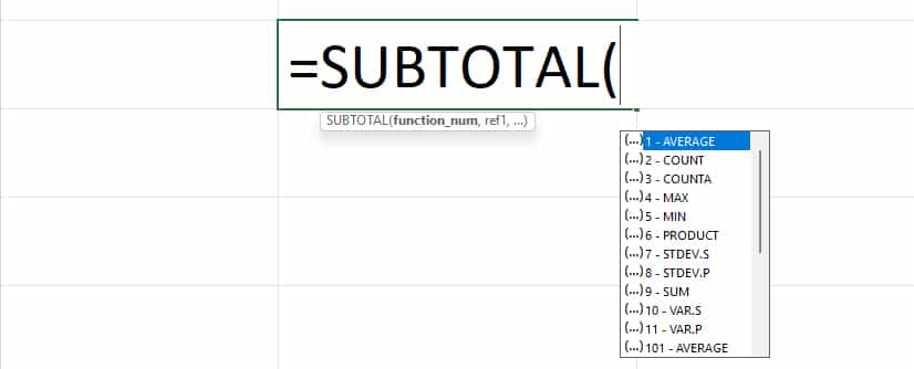
The SUBTOTAL function in Excel is a versatile tool that goes beyond simple addition, offering various calculations like sum, average, count, and more, depending on the function number you choose. It's particularly useful in scenarios like inventory management because it allows you to perform these calculations on filtered data, excluding hidden rows, which is a significant advantage when analyzing subsets of data.

For instance, if you have a list of inventory items with their quantities and prices, you can apply filters based on categories or time frames and use the SUBTOTAL function to calculate totals or averages only for the visible, filtered data. This capability is invaluable for getting quick insights into specific inventory segments without creating separate tables or lists.

The SUBTOTAL function has 1-11 and 101-111 numbers. The former includes hidden cells in its calculations, whereas the latter excludes them, providing flexibility based on your needs. 

This dual functionality allows you to adapt the function to various scenarios, such as adjusting your inventory analysis based on visible data points or considering the entire dataset, including hidden rows​​.

In practice, you could use SUBTOTAL to calculate the total stock value of filtered items, the average price of visible products in a category, or count the number of items in stock within a specific range, adjusting dynamically as filters are applied or removed. This function is not just limited to summing; it can apply any of its 11 different calculations to your filtered inventory data, offering a comprehensive tool for data analysis within Excel​​.

CONCAT Function

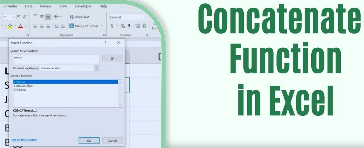
The CONCAT function in Excel is designed for merging text from multiple cells or ranges, creating comprehensive data strings. It's a powerful tool introduced in Excel 2016 as an enhancement over the older CONCATENATE function. 

The CONCAT function can handle a range of cells, not just individual cell references, which makes it more efficient for combining large data sets.

For example:

If you want to merge the first and last names from different cells with a space between them, you will use =CONCAT(A1, " ", B1). This function can also handle different delimiters, such as commas or line breaks, between the text elements you combine. 

If you needed to add a comma and space between words, your formula might look like =CONCAT(A2, ", ", B2, ", ", C2).

One of CONCAT's key benefits is its ability to ignore empty cells automatically. This feature simplifies merging text from ranges that might have gaps. 

However, it's essential to remember that CONCAT doesn't provide a built-in way to specify a delimiter for the combined values, unlike the TEXTJOIN function, which can be used when a common delimiter is needed.

In addition to text, CONCAT can be used to merge numerical values and dates, though it's crucial to use the TEXT function to maintain proper formatting for numbers and dates within the CONCAT formula. For instance, to merge text and a formatted date, you might use =CONCAT("The date is ", TEXT(A1,"mmmm d")).

In inventory management:

CONCAT can be incredibly useful for creating unique identifiers or detailed descriptions by combining information from multiple columns into one. For example, you could combine product codes, names, and specifications stored in separate columns into a single, detailed product description column.

IF and IFS Functions

The IF and IFS functions in Excel allow you to perform conditional operations. While the IF function tests a single condition, the IFS function can evaluate multiple conditions sequentially.

Here's a comparative table that outlines the key differences and uses of the IF and IFS functions in Excel:

The IF function is ideal when you have a single condition to test or when you want specific control over each logical test's outcomes. In contrast, the IFS function is more efficient and easier to read when you have multiple conditions to check, avoiding the complexity of nested IF statements.

VLOOKUP and HLOOKUP Functions

Excel's VLOOKUP and HLOOKUP functions in Excel are designed for vertical and horizontal data retrieval. Here's a detailed breakdown of their functionalities and importance in data retrieval:

VLOOKUP is widely used in various vertical lookup applications, especially when dealing with tabular data where specific information needs to be extracted based on a matching condition. HLOOKUP serves a similar purpose but is designed for horizontal data layouts, making it a crucial tool for retrieving information across rows. 

Both functions are fundamental for data analysis, reconciliation tasks, and streamlining data manipulation processes in Excel.

COUNTIF and COUNTIFS Functions

Excel's COUNTIF and COUNTIFS functions in Excel are essential for conducting conditional counting in datasets, such as customer data analysis.

Here's an overview of how they work and how they can be applied in a practical context:

• COUNTIF Function in Excel: COUNTIF counts the number of cells that meet a specific criterion within a range. Its syntax is =COUNTIF(range, criteria). The function is versatile, allowing you to use logical operators (e.g., >, <, =) for numeric data and wildcard characters (e.g., *, ?) for text data​​.
• COUNTIFS Function in Excel: COUNTIFS extends the capabilities of COUNTIF by allowing you to apply multiple criteria across multiple ranges. Its syntax is =COUNTIFS(criteria_range1, criteria1, [criteria_range2, criteria2], ...). This function is particularly useful when you must simultaneously analyze data based on several conditions​​.

Application in Customer Data Analysis:

• Identifying Customer Segments: You can use COUNTIF and COUNTIFS to segment customers based on various attributes. For instance, in a retail banking dataset, you could categorize customers by balance ranges using IF statements and then apply COUNTIF to count the number of customers within each balance band​​.
• Cross-Reference Analysis: With COUNTIFS, you can perform cross-reference analysis by applying multiple criteria. For example, you could analyze the distribution of customer balances across different regions, identifying how many customers have balances above a certain threshold within each region​​.
• Trend Analysis Over Time: By incorporating time-related criteria, COUNTIF and COUNTIFS can help you analyze trends over time, such as tracking the growth or decline of customer accounts or analyzing regional performance across different periods​​.
• Handling Text and Dates: These functions are adept at handling text and dates. For example, COUNTIF can be used to count occurrences of a specific name within a data range, and with dates, you can use COUNTIFS to count occurrences before or after a certain date or within a date range​​.

AVERAGE, MEDIAN, and MODE Functions

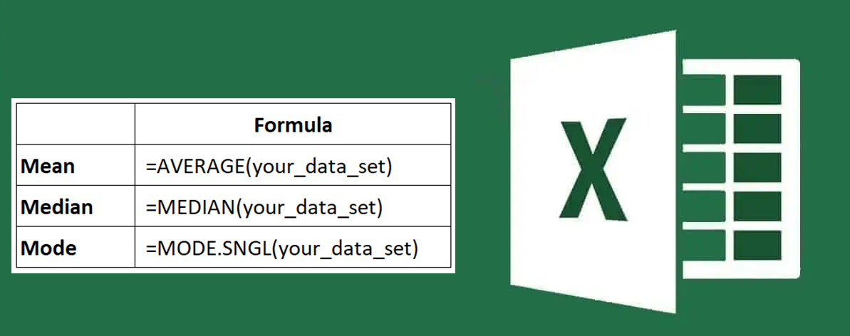
The functions AVERAGE, MEDIAN, and MODE in Excel are fundamental for statistical analysis, particularly in market research or sales data analysis. Here's a summarized table outlining their use cases:

For example, the AVERAGE function can help analyze average customer satisfaction scores in market research. The MEDIAN function is beneficial when you want to find the middle point in data, like the median sale price, which can provide insights without being skewed by extremely high or low values. 

The MODE function can be crucial in identifying consumers' most common preferences or choices, such as their most preferred product features.

TEXT Functions (LEFT, RIGHT, MID)

Excel's LEFT, RIGHT, and MID functions are powerful tools for manipulating text strings, which can be extremely useful in data cleaning and organization tasks. Here's a brief overview of how these functions can be applied:

• LEFT Function: The LEFT function extracts a specified number of characters from a text string's beginning (left side). For example, if you have a string 'ABCDEF' and use =LEFT("ABCDEF",3), the result will be 'ABC'​​.
• RIGHT Function: Conversely, the RIGHT function extracts characters from a text string's end (right side). Using the same string 'ABCDEF' with =RIGHT("ABCDEF",3), the result will be 'DEF'​​.
• MID Function: The MID function extracts characters from the middle of a text string, given a starting position and the number of characters to extract. For instance, =MID("ABCDEF",2,3) would result in 'BCD', starting from the second character and extracting three characters in total​​.

These functions can be particularly useful in various scenarios, such as:

• Extracting specific parts of data entries that follow a consistent pattern (e.g., extracting area codes or extensions from phone numbers).
• Isolating specific information from strings where identifiable characters or patterns surround the desired text.
• Cleaning data by removing unnecessary prefixes or suffixes in strings.

For example, in data cleaning, you might encounter a situation where you must extract just the first name from a full name. If the full name is in the format 'First Last', you could use the LEFT function and FIND to extract the first name. 

Similarly, the MID function can be invaluable if you need to extract data consistently positioned in the middle of strings.

XLOOKUP Function

XLOOKUP is a powerful Excel function introduced as a more flexible and potent alternative to the older VLOOKUP and HLOOKUP functions. The XLOOKUP function searches a range or an array, and then returns the item corresponding to the first match it finds. If no match exists, then XLOOKUP can return the closest (approximate) match. *If omitted, XLOOKUP returns blank cells it finds in lookup_array.

Here's an overview of how XLOOKUP can enhance your data analysis tasks:

1. Simpler Syntax: XLOOKUP requires only three essential arguments: the lookup value, the lookup array, and the return array. This streamlined approach makes it easier to use compared to its predecessors​​.
2. Bidirectional Lookups: Unlike VLOOKUP, which only searches in a left-to-right direction, XLOOKUP can retrieve data to the left or right of the lookup values, offering greater flexibility​​.
3. Enhanced Match Control: XLOOKUP allows for exact matches, approximate matches, and even wildcard matches, providing more control over how your searches are conducted​​.
4. Custom Error Handling: If XLOOKUP doesn't find a match, you can specify a custom return value, which simplifies error handling in your formulas​​.
5. Versatility in Return Values: XLOOKUP can return single values, arrays, or entire rows/columns, expanding its utility in various scenarios​​.
6. Search Modes: You can define the direction of the search, either from the first to the last value or in reverse, adding another layer of flexibility to your lookup tasks​​.

Here are a couple of practical examples where XLOOKUP can be particularly useful:

• Dynamic Two-Way Lookups: XLOOKUP can perform vertical and horizontal lookups in a single formula, making it an excellent tool for two-way lookups where you need to find a value at the intersection of a specific row and column​​.
• Nested XLOOKUP for Multiple Data Sets: You can nest XLOOKUP functions to search across multiple data sets, even on different sheets, which is particularly useful when consolidating data from various sources​​.

PivotTables and Excel Functions

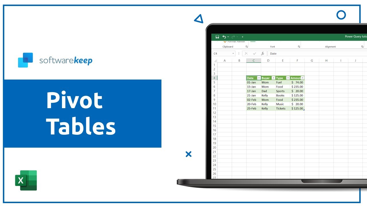
Various Excel functions can significantly enhance PivotTables in Excel, making complex data analysis simpler and more intuitive. Here are some ways to enhance PivotTables with Excel functions and examples of how they can simplify complex data analyses:

1. Slicers for Data Segmentation: Slicers provide a quick way to filter PivotTable data interactively. By adding a slicer, you can filter the data displayed in the Pivot Table based on your selection, making it easier to focus on specific data segments​​.
2. Calculated Fields: You can create calculated fields within PivotTables to perform calculations on your data. For instance, if you're analyzing sales data, you can create a calculated field to determine the profit for each item by subtracting the cost from the sales price​​.
3. Multiple Pivot Tables from One Source: You can create multiple pivot tables from a single data source to analyze different aspects of your data. This can be particularly useful for comparing different data segments side by side​​.
4. Advanced Sorting and Filtering: PivotTables allow for advanced sorting and filtering, including custom sorting and the ability to filter by top 10 values or specific ranges. This makes it easier to focus on your analysis's most relevant data points ​​.
5. Timeline Filtering: If your data includes date fields, you can add a timeline to your PivotTable, allowing you to easily filter data based on periods. This is especially useful for time-based data analysis, such as sales trends​​.
6. Value and Label Filtering: Beyond the basic filtering options, PivotTables support more nuanced filtering techniques, such as value and label filters, enabling you to narrow down your data precisely based on specific criteria or conditions​​.

Dynamic Arrays (FILTER, SORT, UNIQUE)

Excel's dynamic array functions, FILTER, SORT, and UNIQUE, offer powerful data segmentation and organization tools. Here's a brief overview of how these functions can be applied in practical scenarios:

These functions allow for advanced data manipulation in Excel, providing efficient ways to dynamically segment, sort, and extract unique values from your data.

Error Handling (IFERROR, ISERROR)

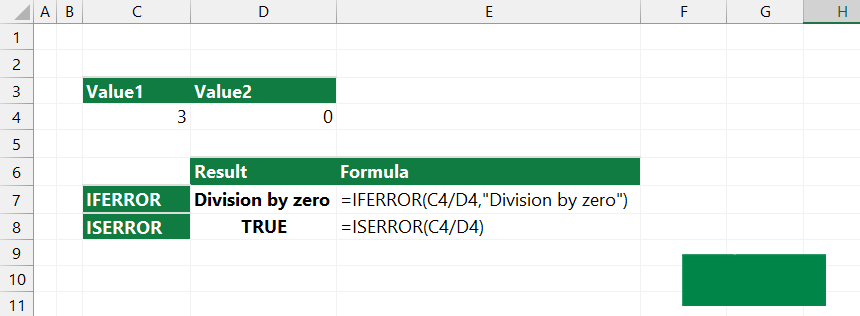
In Excel, the IFERROR and ISERROR functions are pivotal for managing calculation errors, thereby maintaining data integrity. In its pure form, ISERROR just tests if the value is an error or not. It's available in all Excel versions. The IFERROR function is designed to suppress or disguise errors - when an error is found, it returns another value that you specify.

Here's an overview of how these functions work and their applications:

• IFERROR Function: This function allows you to specify a custom output when a formula detects an error. Its syntax is =IFERROR(value, value_if_error), where value is the evaluated expression, and value_if_error is the result returned if an error is detected.
  For example, =IFERROR(1/0, "Error") would return "Error" instead of the default #DIV/0! error. This function is particularly useful for ensuring that your spreadsheets remain clean and user-friendly, avoiding the clutter of standard error messages.
  It's also commonly used with VLOOKUP to handle the #N/A error when a lookup value isn't found​​.
• ISERROR Function: This function determines if a formula results in an error, returning TRUE if there's an error and FALSE otherwise. Its usage is straightforward: =ISERROR(value) checks if value is an error.
  This function is especially useful for preemptively checking for errors across a range of cells. For instance, =ISERROR(1/0) would return TRUE. You can combine ISERROR with IF to provide a specific output when an error is detected, like =IF(ISERROR(1/0), "Error detected", 1/0), which would return "Error detected" in case of an error​​.

These functions are essential for maintaining data integrity and readability in practical applications, especially in large datasets where manual error checking is impractical. They are used in various scenarios, such as financial analysis, inventory management, and data validation processes, to ensure accurate and error-free results.

Final Thoughts

Mastering the IFERROR and ISERROR functions in Excel is crucial for anyone aiming to enhance their spreadsheet skills. These functions are key to managing errors efficiently, ensuring data integrity, and maintaining spreadsheet readability. 

By incorporating IFERROR and ISERROR into your Excel toolkit, you can handle unexpected inputs gracefully and keep your data analysis processes robust and error-free. Now that you understand the importance of these functions, explore them further and boost your Excel proficiency. 

Whether you're a beginner or looking to refine your skills, delving into these functions will elevate your spreadsheet game.

Keep Learning

» How To Use Excel’s DATE Formula Function
» Excel Tutorial for Beginners: Tips You Need to Know
» How to Manage Your Finances With Microsoft Excel
» The Benefits of Microsoft Office for Students and Professionals
» Office 2021 for Home and Business Guide

If you're trying to sort by date in Microsoft Excel, and wondering how to do it, you’re in the right palace.

You’re not alone. Most Excel users rarely enter a date directly in Excel.

Excel sorts data based on the format you choose. So, to use the Date sorting feature properly, you'll need to understand how the DATE FUNCTION works in Microsoft Excel.

Whatever you type in excel, the app will convert into the proper format. If you use Excel's native date sorting functions, your Excel dates will be sorted in Excel's date order.

If your Excel data is not in an Excel standard column, it will default to the next best thing available.

So, let’s dive into sorting by dates in Excel.

Sort Excel by dates

To sort excel by date, do the following:

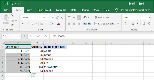
1. Drag down the column to select the dates you want to sort.
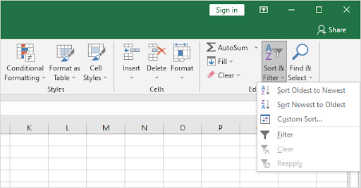
2. Click Home tab > arrow under Sort & Filter
3. Click Sort Oldest to Newest, or Sort Newest to Oldest.

Let’s discuss this process in detail below!

Sort by Date in Excel (Windows and Mac)

Excel dates are easy to sort manually, but Excel’s automatic date sorting often fails. On Excel for Windows and Excel for Mac, you can use the native sort by date function to get the dates in a column sorted properly.

You can also use Excel’s Sort & Filter tool to further manipulate how your dates are displayed, and get more information at a glance. Some Excel versions have a feature that allows you to sort multiple columns by date as well. Alternatively, you can use an Excel macro similar to Multi Column Sort.

Note: This guide is written using Excel 2019, however, the steps apply to various other versions including Excel for Mac, Excel 2016, Excel 2013, and Excel for Microsoft 365.

1. Select the first date in your list, then drag down the column where your dates are to select all of them with the cursor. You may also hold the Shift key and click on the last date to select the entire column.
   
   
2. Go to the Home tab in your Ribbon, located on top of the Excel interface. Here, click on the Sort & Filter icon to expand its options.
   
   
3. Choose either the Sort Oldest to Newest or Sort Newest to Oldest option depending on the desired result. You should immediately see your dates rearrange based on what you selected.

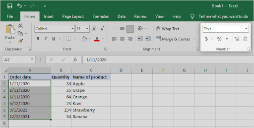
If you notice that your dates won’t change in order, or don’t have the option to sort them as dates, you might have them formatted as text. You can fix this by following the section below.

How To Convert Dates Stored As Text in Excel

Is the sort by date function not working in Excel? Typically, Excel will only sort cells that are converted into a date format. In Excel 2007 and newer, Excel sorts by the data type, you have selected.

If the date sorting feature doesn't work, there's a possibility that your cells are formatted as text. Excel will not sort cells that are formatted as text, so you'll need to convert them into Excel's date format.

1. Select your wrongly formatted dates, and then click on the drop-down menu in the Number section found in the Home tab. The menu should display “Text” or something other than the date.
   
   
2. Select either Short Date or Long Date from the drop-down menu. The formatting of your cells should automatically change, allowing you to sort by date.
   
   

Final Thoughts

Date sorting is one of the most underrated features in Excel, but it’s worth understanding how to use. When you sort by date, you get a different view of your data and see what needs attention quickly.

One more thing

If you’re having other issues with Excel, don't worry! Our Help Center has an article covering hundreds of issues and also provides tips on how to get the most out of the Office. For more information about all things tech, visit our Blog. We hope we can be of help!

For those who want more information, sign up for our newsletter. Get promotions, deals, and discounts from us right in your inbox. Subscribe with your email address below. You'll be the first one notified about our latest news as well as great deals you can't miss out on.

You May Also Like

» How to Add a Trendline in Excel
» How To Lock and Unlock the Scroll Lock in Excel
» How to Edit Legend in Excel

So, if you’re intimidated by the idea of using Microsoft Excel to manage your finances, you’re in the right place.

You will learn how to use Microsoft Excel to manage and save money.

Overview

Managing personal finances is a daunting prospect for most people. But having the right tools can help make it less challenging.

While most people use Excel to track their budgets, manually updating your budget spreadsheet every month is a time-consuming process.

But with the right knowledge of Excel, you can make the process a more seamless experience.

So, today, you’ll learn about how to use Excel to manage your finances to simplify your day-to-day money decisions. With this guide, you can stay on track with your longer-term financial goals.

Why You Need To Budget for Your Expenses

Budgeting is a great way to keep track of your spending, income, and savings. This will ensure that you are on track with your finances and can meet future goals.

For example, I am saving to purchase my first home. Each day, the money I save makes a huge difference. Knowing where my income is coming from and where it's going gives me greater control over my financial decisions.

If you have more than one account for your income and expenses, it's important to track them separately. No matter how much detail you are expecting about your income or spending habits, having an Excel budget will help maintain control over your finances.

Use Microsoft Excel for your financial spreadsheets to access them anywhere with Office 365.

Your spending habits are logged so you can decide where to cut costs. Each month is different because there's more income coming in than out, but it's necessary to track in order to make better decisions.

How To Use Excel for Budgeting

Before you can begin creating your ultimate budgeting spreadsheet, you need to get access to Excel. If you don't own the application yet, check out our store and purchase Microsoft Excel. Alternatively, you can install Microsoft Excel from the Office 365 app store.

Step 1. Set Up the Budgeting Spreadsheet

Setting up your workbook for finances is easy. First, list all of your bills on one side. Try adding as many monthly expenses as possible. You should also include the amount of money spent, and the date of the expense. It seems easy enough; just start with what I have done below:

Of course, you can expand this further by adding more details, such as the payment method, notes, and more. This is your spreadsheet, get creative and customize it for your needs!

If you want to keep things super simple, you can stop here. This is already a great budgeting sheet that lets you keep track of things with ease. However, you can take it several steps forward by implementing functions.

Step 2. Add Excel Functions to the Sheet

If you know how to use SUM, then it is easy to implement a cell for your total spendings, income, or savings.

The first step is to create a formula that will pull up the total amount of your bill from your list of bills on the left side. You can do this by using the SUM function, which is one of the basic features of Excel.

Here’s how to get the total working:

1. Decide on which cell you want to hold your total, and select it.
2. Type in the following formula: =SUM(B2:B9). If you’re not following along with our sheet, make sure to replace the cells with the first and last cell in your spreadsheet.
   
   
3. Press Enter. You should see the total of your money immediately displayed. This total will automatically and accurately calculate a new total as you spend more or gain more income during the month.

Step 3. Get Better Insight by Sorting Your Data

You can easily see which of your expenses are the highest, by simply sorting the spreadsheet. For example, maybe your cable television bill is higher than it really should be.

From there, you can get a sense of what you might need to do — whether that’s negotiating a better price on your package, or cutting the cord entirely.

1. Highlight your cells that hold currency data. When done, switch to the Home tab in your ribbon, and click on Sort & Filter, and then select either Sort Smallest to Largest or Sort Largest to Smallest.
   
   
2. A warning may appear on your screen. Here, we recommend selecting the “Expand the selection” option to ensure everything moves properly in your sheet.
3. Voila! Your expenses are now organized. This is one of the first steps in learning how to make better financial decisions in the long run.
   
   

Step 4. Format Your Spreadsheet for Readability

I recommend adding some visual indicators to your budget workbook to make it easier to read and understand at a glance. For example, if a number is lower than zero (meaning you spent more on it than you had budgeted), add red borders around the cell where that number appears.

You can also create layouts by differentiating between your headers and entries. There’s no right or wrong way to do this, so I’ll show my personal shading as an example below:

You can replicate this look by utilizing the Font Color, Fill Color, and Borders in the ribbon's Home tab.

Additionally, you can change fonts and format text through the same tab as well.

Step 5. Visualize With a Pie Chart

It's hard to notice details when you're just looking at raw numbers, and that fear holds people back from actually taking action on their budgets - which is why Excel has graphs!

They make it so much easier for you to see trends over time with a visual representation and they show where your money goes too.

I have always been intimidated by spreadsheets full of rows upon rows or columns. Thanks to the charts found within Microsoft Excel, anything can be more easily understood as well as broken down into manageable pieces.

The charts and graphs in the program help you see exactly where all of your money is going, making it a lot easier for me to save up some dough!

At first, seeing that I spent $30 USD on various online subscriptions in a month doesn’t seem that alarming at first glance. After seeing how this amount looks in proportion to what

I spent on my groceries, I knew that it’s time to review what services I’m subscribed to. This simple pie chart saved me almost $20 USD every month.

The 5 Best Finance Tracking Templates for Excel

Many people prefer to work with templates as they save an immense amount of time. But finding the right template for your needs can be a real nightmare. Here are 5 of the best finance tracking templates for Excel:

1. Simple Monthly Budget Template by Microsoft

If you have never worked with an Excel spreadsheet before, then you will find this budget template incredibly easy to use. This workbook will help you see the cash flow in your life. Complete these three pages and then compare them to understand where all of your money is going!

The main page shows a snapshot of how much money came into, went out from and remained on hand at any given time over the course of one month. The next two pages are Monthly Income and Expenses.

You can update the pages according to what's coming in or being spent throughout this year.

Download the Simple monthly budget template here. (Free)

2. Household Expense Budget Template by Microsoft

Do you share payment responsibilities with other people and find it difficult to keep track of who has paid what? Introduce the budgeting template into your lives so that all roommates are involved in this process.

The customizable spreadsheet shows how payments will be spread amongst everyone, which is great for adjusting responsibility as needed.

Do you know how it's difficult to keep track of your expenses when you have an irregular income? For example, if one person pays the hydro bill while another pays for groceries. Well, this is where a roommate payment template comes in!

The free customizable spreadsheet helps make sure everyone knows who paid what and there are no more disputes over who should pay next time because everything is clear on paper (and easy to access or update online).

Download the Household expense budget template here. (Free)

3. Monthly College Budget Template by Microsoft

College is a lot of responsibility, and financial decisions can feel daunting. Thankfully this template has all the tools you need to make smarter financial choices!

The customizable graphs will allow you to visualize your spending habits at any time, while also giving an overview of how much money remains in your account each month.

Create multiple tabs for different types or goals so that it's easier for yourself when managing finances with schoolwork on top of everything else going on during college.

It'll be like having a personal assistant always right there, guiding you every step of the way.

Download the Monthly college budget template here. (Free)

4. Tax Expense Journal Template by Microsoft

This template is the perfect way to simplify your taxes. With a sophisticated design and tracking features, you'll be able to keep an eye on every expense that needs attention for tax purposes.

The sleek table design automatically updates as you make changes — just like other templates in this list! You can also add more rows with ease, or attach useful notes, dates, descriptions, and totals at any time of year.

At the bottom of each page, there's always a “Total” amount displayed so it's easy enough to make smart decisions about where your money goes before filing!

Download the Tax expense journal template here. (Free)

5. Monthly Company Budget Template by Microsoft

Keeping track of expenses and income is necessary for individuals, but it's also crucial to a business. This template lets you log in all the money that comes into your company as well as everything going out.

It has features that help with budgeting and forecasting — such as an easy-to-read bar graph on the first page, which breaks down how much was spent over a time period.

You'll be able to see how much has come in vs what was predicted, as well as seeing all expenses broken out into subcategories like personnel or operating costs. This way, no detail gets missed.

While logging information can often feel tedious, this intuitive template is designed specifically to keep things easy-going without compromising quality.

Download the Monthly company budget template here. (Free)

Final Thoughts

That’s it: You now know how to manage your finances with Microsoft Excel.

If you were having difficulties in managing your budget before, just follow this guide to track your spending.

Now, it’s your turn.

If you’d like to know more about Excel, visit our Help Center for more Excel topics.

Also, sign up for our newsletter below to get our updates on new guides, promotions, deals, and discounts.

Keep Learning 

» Expense Record & Tracking Sheet Templates for Excel
» How to Calculate CAGR in Excel
» Save Hundreds of Dollars With These Google Chrome Extensions

Have you ever tried to insert a PDF into Microsoft Excel, but failed to do it? We know — it's not easy, and it usually ends up in frustration.

With this article, you can learn how to do it easily!

We'll teach you how to create a new workbook in Excel for your PDF file so that it will show up as an object on the spreadsheet, and then we'll show you how to get the data from your PDF into cells of your spreadsheet.

You can even open a PDF file in Excel and begin editing its contents right away.

Sounds good? Let’s get started.

Why Are PDFs in Excel Useful?

Portable Document Format (PDF) allows you to store, share and open documents without any changes in the data regardless of the program used. Thanks to Excel, it's now possible for users to organize their information by inserting a PDF file into an excel spreadsheet with ease.

Besides this capability, PDF files can also be extracted directly from that document so they are visible on your screen for use within other programs such as PowerPoint or Word.

We will walk through quick and simple steps on how to insert a PDF file into an Excel workbook either as an object or link using our guide below.

When To Insert a PDF Into Excel

PDF has a lot of benefits for Excel. It's easy to view and share, so it'll stick around because everyone can read PDF files while they're still in the same formatting as when you originally created them.

The following are some situations where you would want to embed PDF into your Excel spreadsheet:

• Preparing a report: The best way to make a spreadsheet engaging is by adding charts and tables. It’s easier to read data that way, rather than when it's all written down on an Excel spreadsheet. If your report includes lots of detail, attach a PDF with more information.
• Having all sources in one document: When you have a very long report, make sure that all the sources are in one place. You can use a PDF for this. Save time as you don't need to search for a different file before going back into your spreadsheet.
• Creating a product catalog: When you are making a product catalog, you can add more details to each of your products by inserting a PDF file. This keeps the catalog tidy and usable for formulas, but gives you direct access to more details.
• When presenting the entire worksheet: It’s easy to directly copy-paste a section of a PDF file into the Excel workbook. When you need to work with the whole workbook, it’s better to copy and paste the PDF file including copies of scanned receipts into Excel.
• Focusing on crucial information: If you want to see only the most important information on your Excel worksheet, then you can insert a PDF file to store other information. You can also refer to other comments or info in that file when needed.

How To Insert a PDF Into Excel

Embedding a PDF into an Excel document can seem challenging at first but is actually quite easy with these steps below!

How to Insert PDF into Excel - from Excel as an Object

The quickest way to insert PDF files into Excel sheets is via the software itself.

1. Open the Excel document that you wish to insert a PDF file into

2. Click 'Insert' > Object... > From File

3. Locate the PDF and click 'Ok'

How to Insert PDF into Excel - from Excel as a Picture

1. Similar to the last step, have the Excel file open

2. This time, click 'Insert' > Picture > Picture from File...

3. Locate and double-click on the PDF you wish to insert into Excel

Voila! That's done. Inserting content from a PDF file into an Excel sheet could not get any easier than this.

Similarly, you can also choose other file formats, such as images to place inside your Excel files.

There are different other ways in which you can put a PDF file into Excel. Review your options and see what works for your unique needs.

Option 1. Embed the PDF Into Excel

The classic way of adding a PDF file into your Excel worksheet is by simply embedding it into the workbook itself.

This gives you easy access to anything included in the PDF and your workbook at the same time. You can even link data between the files.

1. Open the Excel spreadsheet that you want to embed the PDF file into.
2. Click on the Insert tab from the Ribbon menu on top of your interface.
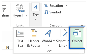
3. On the far right, locate the Text group command, and then select Object from the context menu.
   
   
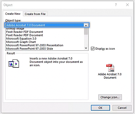
4. Once the dialogue box appears, click on Create New, and then select Adobe Acrobat Document from the list.
   
   
   
5. If you’d prefer the PDF content to be invisible but still remain accessible, select the Display as icon checkbox.
6. Click OK. Select the PDF file that you want to insert from the menu.
   
   
   
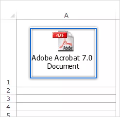
7. If selected, the document will appear as an icon that can be dragged to any position within the spreadsheet.

To insert more PDF files into your spreadsheet, repeat the same process. Note that this method doesn’t only insert the first page of your PDF document.

Instead, it embeds the whole object, including multiple pages.

Option 2. Use the "Link to File" Feature

A file size constraint is a downside of embedding a PDF into the Excel worksheet to share with others.

The best way to avoid this problem and maintain high quality, without increasing the file size, is by linking directly from the source file.

1. Open your preferred spreadsheet, and then click the workbook cell that you want to insert the PDF object into.
2. Next, switch to the Insert tab in your Ribbon menu, and click on Object in the Text group similarly as before.
3. Click Create from File on the Object dialogue box. Make sure you select the Link to File checkbox. Optionally, select the Display as Icon checkbox to secure the content of your PDF.
4. Now, click on Browse, and select the PDF File to be linked. Click Insert, and finally, click on OK. The PDF document will appear as an icon inside your Excel workbook.

By linking your workbook with the source PDF file, your workbook will essentially become a live report.

This means any changes made on either end of this equation are reflected in real time, so you can see exactly what is happening without having to constantly refer back and forth between them.

However, only do this if a backup of both Excel and the object type you're linking have been stored on one drive for safekeeping — you don't want something important being deleted!

Option 3. Insert PDF Into Excel 2013

Why not create a spreadsheet? It's easy to do.

The easiest way we recommend for inserting a PDF file into Excel 2013 is using these quick but straightforward steps. You can find them on TikTip, your one-stop shop for any Excel tips and tricks, even for older versions.

How To Adjust the Inserted PDF File in Excel

One major drawback of inserting the PDF file into an Excel spreadsheet is that it does not sort or filter with cells.

However, there are ways to make your newly embedded document fit in the cells without altering its content — here's how!

1. Right click on the PDF file you have inserted, and then click the Format Object option on the context menu.
2. Next, the Format Object dialogue window opens. Click on Properties, and then select Move and Size with Cells from the given options.
3. Click OK to adjust the file to your preference.

If you want to filter or hide cells inside your workbook, then a similar action will apply to the PDF file.

How to Insert PDF into Excel - with Third-Party Tool

You can also insert a PDF into excel using a third party tool like Smallpdf. It even makes work with PDF easy, including the transfer of file formats, to and from this universal file.

Furthermore, their OCR technology can now help you convert PDF to an editable Excel file.

As such, you can now convert PDF to Excel files and merge your sheets together into one, to manage and edit them easily.

To do so:

1. Go to the PDF to Excel tool on our site

2. Drag and drop your PDF to convert to Excel

3. Download your file, upload to Google Drive or Dropbox, or even share via email

How To Review Your PDF in Excel

After inserting your PDF file into Excel, you can then review the image through these simple steps:

1. Right-click the image on the Excel workbook and select Acrobat Document Object.
2. Click Open. The PDF document opens in a different Adobe window, where it can be viewed properly.
3. Once you’re done reviewing the PDF, click on Save from the Quick Access Toolbar and save any changes. The attached PDF appears as an attachment on your Excel spreadsheet.

How To Rename the Inserted PDF

There’s a way to make your PDFs more searchable and easier to find. By default, Acrobat gives the PDF file you embed into an Excel spreadsheet generic document name such as "Adobe Acrobat Document".

Don't let this stop you from giving it a clever title, follow these steps!

1. Right-click on the PDF file on your Excel workbook, and then click Acrobat Document Object from the context menu. Select the Convert option.
2. Check the Display as Icon box, and click on Change Icon.
3. A Change Icon dialog box appears. In the Caption field, type the desired name of the PDF file to suit your preference.
4. Click OK to save the changes. It’ll reflect inside your Excel worksheet.

Still here?

Visit our Help Center to get access to hundreds of articles covering hundreds of topics, and with tips on how to get the most out of your system.

Want more? Sign up for our newsletter to get promotions, deals, and discounts from us right in your inbox. Subscribe with your email address below.

Keep Learning

» How to Create Excel Header Row
» How To Use “If Cell Contains” Formulas in Excel
» How to Edit Legend in Excel