Ready to revolutionize your web development process? Our guide explains the significance of RACI templates and guides you through their implementation. Uncover the art of efficient delegation and empowerment. Join us as we unpack the why, how, and boundless benefits of integrating RACI templates into your website projects. Your journey to enhanced collaboration starts now.
In website development, unclear roles can lead to a tangle of confusion and missed opportunities. Imagine a project where nobody knows who's in charge of what – deadlines slip, tasks fall through the cracks, and finger-pointing begins. This is where the RACI framework rides in like a hero.
RACI stands for Responsible, Accountable, Consulted, and Informed – a fancy way of sorting out who does what in a project. It's like a traffic signal for tasks: who's driving, who's keeping watch, who's advising, and who's just in the loop.
Role clarity is where the magic happens. With RACI, everyone knows their part in the play. This means less squabbling over whose job is whose, and more energy directed at the actual work. Reduced conflicts are like a breath of fresh air. When folks aren't stepping on each other's toes, collaboration blooms.
Think about a smoothly oiled machine – that's what RACI can do for your project. By designating roles, you minimize the merry-go-round of decision-making. Things don't stall waiting for approvals. Plus, real-life numbers back this up: teams using RACI report faster task completion and fewer hiccups.
Take this example: A website launch. The developer, Designer Dan, is responsible for coding, while Content Chris is accountable for writing. Marketing Mary is consulted on branding, and CEO Alex is kept informed. With RACI, everyone's in sync, and the launch goes off without a hitch.
Ever heard of RACI templates? They're like the superglue that holds web projects together, ensuring smooth sailing from start to finish. Here's the lowdown on why they're a total game-changer:
Picture this: a project derailed by finger-pointing and confusion. RACI templates toss that chaos out the window. They assign crystal-clear ownership for each task so everyone knows who's driving the ship. No more "I thought you were handling that!" moments – just pure clarity.
Defined roles mean defined actions. RACI templates lay out who's doing what, streamlining the entire process. Tasks flow seamlessly, like a well-choreographed dance. With everyone tuned into their roles, bottlenecks vanish, and productivity soars.
Waiting for approvals can feel like watching paint dry. RACI templates introduce the right folks at the right time, slashing decision-making time. It's like having a VIP pass to quick choices – critical for staying on track.
Ever felt like important updates get lost in the shuffle? RACI templates put an end to that. They improve communication by defining who needs to know what. Everyone stays in the loop, ensuring no detail is left in the shadows.
Creating and using RACI templates might sound like tech-speak, but trust us, it's simpler than assembling IKEA furniture. Here's your no-nonsense guide to making it work for your website projects:
Imagine your website project as a puzzle. Step one is sorting out the pieces. List down every task and process your project involves. This could range from designing and coding to content creation and testing.
Now, let's divvy up the tasks. RACI roles are like assigning seats in a theater – everyone knows where they belong. Break it down like this:
Like any good plan, you need to jot it down. Create your RACI matrix – a chart showing roles against tasks. It's like your project's roadmap. Sharing it is vital. Think of it as a recipe everyone follows for a fantastic dish.
Step 1: List Roles and Tasks
Think of roles as actors and tasks as scenes. Who's the main character for each scene? Note it down.
Step 2: Match the Players
Assign roles (R, A, C, or I) to each task. Who's leading, who's supporting, and who's just observing?
Step 3: Team Approval
Get your squad's nod. Are the roles aligned with each person's strengths? Adjust if needed.
Step 4: Core Stakeholder Check
Show it to the big players. Are they on board? It's like a script reading – everyone agrees before the show.
Step 5: Keep It Handy
Stick your RACI chart where all can see. It's like the project's map – nobody gets lost.
Implementing RACI templates isn't a one-and-done deal – it's more like nurturing a bonsai tree. Here are the tried-and-true strategies for making the most out of this game-changing tool:
Regular Updates: Keep It Fresh
Think of your RACI matrix like a living document. As your project morphs and grows, your roles might too. Don't let your chart gather dust – make sure it's updated to reflect the current state of play. It's like tuning an instrument for perfect harmony.
Clear Communication: No Secrets Allowed
Ever played telephone? In project land, miscommunication is no game. Keep everyone on the same page by sharing your RACI matrix far and wide. This isn't a secret recipe – it's the recipe everyone should be following.
Training and Familiarity: RACI Jedi Training
You wouldn't drive a car without learning the ropes, right? Same goes for RACI. Train your team so they're RACI rockstars. Explain the ABCs of who's doing what and why. It's like giving everyone a superpower to make projects soar.
You've got a website project on the horizon – and RACI templates are your secret weapons. But wait, what are these templates and how can they turbocharge your work? Let's break it down:
Creately is your creative haven. They offer an editable RACI matrix template, giving you the power to plan your website launch like a maestro. You'll orchestrate a harmonious project symphony with roles assigned to planning, designing, coding, testing, reviewing, and launching.
WPS Office is all about efficiency. Their RACI templates are your compass to streamlined projects. They connect you with quality templates that elevate your game. From planning to execution, expect boosted productivity with their user-friendly tools.
Miro's RACI Chart Template is your ticket to a confusion-free project voyage. This tool acts as your captain in the sea of roles and responsibilities. It keeps your team on track, ensuring everyone knows their part. A vital management tool for smooth project sailing.
Figma brings customizability to the RACI game. Their RACI Matrix allows you to manage your projects like a pro. Assign responsibility for every task, milestone, or decision. Want to try before committing? FigJam offers a free taste of their potent tools.
ProjectManager has your back in mapping your stakeholders. Their free RACI matrix template ensures that every member knows their role in your project performance. By using this tool, you pave a clear path for collaboration and success.
In the dynamic world of website development, RACI templates stand as the beacon of organization and efficiency. They untangle the web of tasks, roles, and responsibilities, providing a clear roadmap for success. By implementing RACI templates, you unlock the power of seamless collaboration, swift decision-making, and precise communication.
Don't let the chaos of undefined roles hinder your project's potential. Embrace RACI templates as your guiding light to streamlined workflows and reduced conflicts.
If you have a second, please share this article on your socials; someone else may benefit too.
Subscribe to our newsletter and be the first to read our future articles, reviews, and blog post right in your email inbox. We also offer deals, promotions, and updates on our products and share them via email. You won’t miss one.
» Top 51 Excel Templates to Boost Your Productivity
» How To Create Your Own Custom Templates in PowerPoint
» 5+ Templates for Excel to Keep Track of Your Fitness
In a world overflowing with information, having a well-structured table of contents is a game-changer. Whether you're a writer, a student, or a professional, an intelligently crafted table of contents can significantly improve the readability and navigability of your work. Say goodbye to confusion and disarray – we're here to help you streamline your content organization.
A well-crafted table of contents brings many advantages that considerably enhance your reading experience. Imagine diving into a book without any clear indication of its structure or what each chapter entails – it would be like wandering in the dark.
The table of contents is your guiding light, offering an immediate glimpse into the content's layout and enabling you to locate what you seek swiftly.
When it comes to table of contents templates, the variety can be both exciting and overwhelming. These templates are like blueprints for organizing your content, tailored to different needs. Let's dive into some common types and how they can benefit you:
In the digital age, a treasure trove of table of contents templates awaits you online. Whether you're embarking on a book, project, or report, these platforms offer various customizable options to suit your needs. Here's where you can discover top-notch templates:
Your creativity's best friend. Explore Canva's versatile collection of table of contents templates that seamlessly adapt to your book, report, or project, elevating your content's visual appeal.
Dive into Visme's guide, showcasing 40 diverse template designs for a table of contents. These templates aren't just standalone – they seamlessly integrate into multipage projects.
Instantly access the perfect table of contents templates in formats like Word, PowerPoint, and Photoshop – all free! A single click grants you professional design for your content.
Elevate your publication's structure with Flipsnack's professionally designed table of contents templates. Present your content in a well-organized manner.
Download professionally designed table of contents template examples here. You'll find a variety of blank index page layouts in formats like DOC and PDF.
A table of contents template acts as your guide. It's a list of sections, chapters, titles, or brief descriptions, all alongside their corresponding page numbers.
Editing made easy. Customize table of contents formats for projects, magazines, and more online, achieving a polished graphic result without fuss.
Remember, the source matters. Opt for reputable platforms like Microsoft Office, Canva, and more to ensure your template's quality and compatibility. A well-structured table of contents starts with a reliable template, setting the stage for your content's success.
Customizing and implementing table of contents templates can feel like crafting a tailor-made suit for your content. Here's how to make it your own and seamlessly integrate it:
Step-by-Step Customization:
Align with Theme and Purpose:
Seamless Integration:
Remember, the goal is cohesion. Your table of contents is a guidepost, so make it a smooth transition for readers. With customization tailored to your content's personality and purpose, the template extends your creation, enhancing navigation and engagement.
Consistency, evolution, and user-friendliness are the pillars of a stellar table of contents. Here's how to nail it:
Maintain Consistency
Update as Content Evolves
User-Friendly Formatting and Design
In the world of content organization, well-crafted table of contents templates are your allies. They streamline navigation, save time, and enhance readability, ensuring readers embark on a seamless journey.
Utilizing templates like those offered by Canva, Visme, and more, you can effortlessly structure your content to match its purpose and tone. Remember, maintaining consistency, updating as your content evolves, and prioritizing user-friendly design are the cornerstones of an effective table of contents.
So, embrace these insights and embark on a new organized and engaging content era.
If you have a second, please share this article on your socials; someone else may benefit too.
Subscribe to our newsletter and be the first to read our future articles, reviews, and blog post right in your email inbox. We also offer deals, promotions, and updates on our products and share them via email. You won’t miss one.
» 10 Free Excel Templates Project Management: Stay Organized and on Track
» Free Expense Tracking Worksheet Templates (Excel)
» 5+ Templates for Excel to Keep Track of Your Fitness
Unleash your creativity, elevate your content, and leave a lasting impression. Embark on this exploration with us as we delve into the world of cutting-edge design possibilities, ensuring your presentations stand out in an ever-evolving landscape. Embrace the future of presentations today!
In a world where presentations are a cornerstone of effective communication, AI-powered PPT templates emerge as a game-changing innovation. These templates, infused with artificial intelligence, elevate the art of presentation design to new heights, ensuring your ideas resonate powerfully with your audience.
But what exactly makes AI-powered templates worth embracing?
When it comes to crafting captivating presentations, harnessing the power of artificial intelligence can be a game-changer. Here's how the top 7 AI PPT template makers are reshaping the landscape of presentation design:
Imagine effortlessly generating templates that fit your exact needs, whether for papercraft, packaging, or learning materials. TemplateMakerX makes this a reality with its user-friendly platform. Here's how it works:
SlideGenius AI, a prominent presentation design agency, has been at the forefront of transforming presentations into compelling narratives since 2012. Boasting a team of over 150 full-time experts, they've served an impressive roster of 4,000 clients worldwide.
Imagine a tool that effortlessly crafts and refines presentations using cutting-edge Generative AI. That's exactly what Plus AI offers. It's a game-changer within Google Slides, empowering users to generate and edit slides like never before.
Your Personal Presentation Assistant:
Think of Plus AI as your personal presentation assistant powered by AI magic. It's as if you have a creative companion that understands your ideas and transforms them into polished slides. The process is simple: start with a prompt, watch the AI weave a customizable outline, and witness it transforming into slides within minutes.
Versatile Customization at Your Fingertips:
What's remarkable is the level of control you have. You can easily modify the content's tone or remix the slide layout to suit your needs. Plus AI even goes the extra mile by offering a customizable outline that lays the foundation for your presentation. Want a specific visual theme? You got it. This tool seamlessly integrates with Google Slides and PowerPoint, ensuring platform flexibility.
Highlights of Plus AI's Power:
Beautiful.ai isn't just another presentation tool; it's your intelligent companion in crafting compelling narratives. The uniqueness lies in its ability to be more than a tool – it's a smart assistant that learns your preferences and tailors suggestions accordingly.
Intuitive Enhancements at Your Fingertips:
Imagine a tool that understands your presentation needs as you shape them. Beautiful.ai's genius lies in predicting what you need and offering suggestions for enhancements. This predictive capability revolutionizes design by streamlining the process and eliminating the guesswork, giving you more time to focus on the message.
Voice Narration for Engaging Presentations:
But the innovation doesn't stop there. Beautiful.ai introduces a voice narration feature, adding an extra layer of engagement. Envision being able to narrate your slides, infusing your unique voice into the presentation. This personal touch becomes particularly powerful for remote presentations, bridging the gap in personal connections.
Key Highlights of Beautiful.ai:
Meet Slidebean, the game-changer in the world of presentation creation. This web-based tool flips the traditional approach on its head, making the process effortless and impactful.
Simple Creation, Powerful Results: What sets Slidebean apart is its remarkable ability to separate the process of content creation from slide design. This means you can channel your energy into shaping your message, while Slidebean handles the design intricacies, resulting in presentations that capture attention.
Design Power for Everyone: Slidebean caters to small to medium businesses, bridging the gap for those without dedicated design teams. It doesn't matter if you're not a design whiz – this tool equips you with the means to create professional-looking slides effortlessly. The secret lies in its treasure trove of design templates, premium fonts, and exquisite color palettes.
Beyond Traditional Tools: Slidebean is more than a substitute for traditional tools like PowerPoint or Keynote; it's an upgrade. It empowers users to craft presentations that transcend the ordinary, leaving a lasting impact on audiences.
Key Features of Slidebean:
Meet Tome, the presentation creator that goes beyond the ordinary. It's not just about crafting slides; it's about empowering users with a collaborative AI assistant that designs engaging presentations from the ground up.
The Power of AI Understanding:
Tome leverages the prowess of OpenAI's ChatGPT and DALL-E 2 technology to grasp your needs and generate content that resonates with your audience. It's like having an AI co-pilot that understands your intentions and brings them to life.
Seamless Design, Endless Possibilities:
Tome isn't just about tools; it's about understanding. With ready-made templates, AI-crafted text and images, plus a variety of multimedia tools, it equips you to design presentations that captivate. But here's the magic: you tell the AI what you want, and it does the heavy lifting. This transforms the design process into a breeze, sprinkled with a dash of fun.
Tome's Stellar Features:
Enter Synthesia, the AI presentation maker that captures attention with its blend of simplicity and innovative features. This tool is all about making presentation creation effortless and impactful.
AI Avatars for a Personal Touch:
One of Synthesia's standout features is its ability to let you create your very own AI avatar. Imagine adding a touch of personal flair to your presentation by introducing your virtual self. This not only engages your audience but also makes your presentation more memorable.
Creating Excellence, No Expertise Needed:
Don't fret if you're not a design whiz. Synthesia levels the playing field by offering many professionally designed video templates that serve as starting points. From there, customization is a breeze, ensuring your presentation fits your specific requirements perfectly.
Versatility for All Audiences:
Synthesia caters to presentations of all scales, whether small team meetings or grand audience gatherings. Its user-friendly interface, personalized avatar feature, and customizable templates ensure your message resonates with impact.
Key Synthesia Features:
Choosing the right AI PPT template maker can significantly impact the quality and efficiency of your presentations. Here's how to ensure you make the perfect selection:
In the dynamic landscape of presentations, embracing AI-powered tools marks a pivotal step toward innovation and excellence. The infusion of AI prowess into design and content creation is transforming how we communicate ideas.
The future holds limitless possibilities as we bid farewell to mundane designs and welcome a new era of visually captivating presentations. With AI at our side, we're equipped to craft narratives that resonate, captivate, and leave lasting impressions on our audiences.
So, let us embark on this exciting journey, where AI becomes our creative ally in shaping presentations that stand at the forefront of impactful communication.
For more such articles subscribe to our newsletter and be the first to read our future articles, reviews, and blog post right in your email inbox.
» 11 Best Microsoft PowerPoint Alternatives and Comparisons
» 10 Best Microsoft Visio Alternatives and Competitors
» 10 Best Fonts for Microsoft Excel
» How To Use PowerPoint Design Ideas: A Complete Guide
» 7 Tips to Improve Your Next PowerPoint Presentation
At the same time, however, the increased digitization of systems and processes comes with an ever-growing price tag that weighs on margins before eventually reaching a point when they are no longer worth it.
This is further aggravated by the shift towards a software-as-a-service and subscription-based pricing model, which means that businesses don’t own the tools they purchase and will incur expenses for using them, either on a monthly or yearly basis.
All of this necessitates an IT cost optimization strategy for organizations big and small to ensure costs don’t escalate uncontrollably and that all IT spends deliver value. This article covers a few tips and best practices for effectively conducting the same.
Any cost optimization initiative begins with a clear understanding of the subject matter at hand and its various factors. In the case of an organization’s tech infrastructure, getting started with a comprehensive IT audit is recommended.
This includes assessing the hardware, software licenses, and maintenance expenses, along with identifying any underutilized or redundant resources, to best guide the cost optimization process.
Such audits should preferably be undertaken by an experienced IT professional or an external software development agency for unbiased and objective reporting of relevant facts and insights.
It is worth noting that there is often more to IT cost optimization than the prices of different applications, and questions such as how much does training cost? Or how the learning curve looks is valid and should be part of the broader equation.
Following a thorough audit, an organization should have a clear map of its broader IT infrastructure, including its top cost drivers. For most businesses, software licenses and keys are likely to lead the way in this regard, making it the right place to start the optimization process.
The audit report should provide a slew of insights about utilization rates, idle times, and more pertaining to each software license, which can unveil cost-saving opportunities, either by surrendering certain licenses or putting off the acquisition of additional licenses.
This can also spur exploration into alternative solutions at a cheaper price or one that is completely open-source and thus free. All in all, this is an area that can drive significant cost savings for organizations when done right.
The benefits of consolidating purchasing power seem fairly obvious in almost all settings, and in the case of IT products and solutions, it mainly helps businesses better negotiate with vendors and sales teams, backed by higher order quantities and purchasing power.
In addition, a centralized team in charge of procurement can institute various workflows to ensure the company’s dollars go the extra mile. It further reduces duplication, resulting in impossible standardization and economies of scale, with individual teams striking out on their own.
There is no denying that centralized procurement saves time and money, with many other benefits, but it is not without its share of drawbacks.
The main one is that it is more akin to centralized planning, as opposed to a free market, where individual teams and their managers choose the tools that best suit their requirements. Strictly speaking from a cost perspective, however, centralization works the best.
In recent years, as IT started playing an increasingly crucial role in businesses and made up a significant chunk of costs, a new body of knowledge has since emerged aimed at effectively managing IT assets with ITAM Software and deriving the most from them.
There are plenty of tried-and-tested best practices in this regard, enough to cover an entire textbook.
For the sake of this article, we’re just going to leave it at maintaining an up-to-date inventory of all software and hardware assets, tracking their life cycles, and ensuring their prompt retirement, renewal, or disposal, as required.
IT cost optimization is an ongoing process that requires regular tracking, assessment, and audits to aid in informed decision-making. The goal is to show continuous improvements in regard to reducing costs, adapting to changing technologies, and aligning IT investments with business objectives.
A slew of objectives, key results, and key performance indicators have since emerged for this very purpose. This includes the likes of price reductions / hard savings, cost avoidance / soft savings, total cost of ownership, and return on investment (ROI), among others.
For example, if the goal is to achieve maximum efficiency with your Zoom licenses, the optimization metrics would include the price reductions won by the procurement team while negotiating with Zoom’s sales team, followed by eliminating wastage by tracking usage metrics on a regular basis.
In the end, the goal of IT cost optimization is to reduce variances between planned and actual expenses on IT infrastructure within an organization. Using KPIs and OKRs helps take a broader view than mere variances, helping better identify problem areas so that corrective actions can be taken accordingly.
Organizations can do several other things to keep IT expenses within budget while hitting other goals and objectives such as strategic alignment, return on investment, and driving efficiency through technology.
For example, Blender is just as good, if not better than premium solutions such as AutoDesk Maya and Wings 3D. Similarly, MySQL and MariaDB do a fairly robust job when compared to the likes of Oracle Database.
Final Words
IT cost optimization is a relatively new field that continues to evolve as new challenges and requirements surface. As of now, it entails an interdisciplinary understanding of IT, management, and accounting to add value to a business, but is quickly turning into a specialized field in its own right.
In this article, we’ve aimed at providing a brief primer on this topic, but as discussed above, in order to cover the true length and breadth of this topic, even a large textbook is barely enough. This, however, should set the stage for most small businesses to optimize their IT expenses going forward.
]]>Get ready to unlock Excel's mathematical prowess and become a master of square roots in Excel. Let's dive in and discover the power of formulas for precise and efficient calculations.
Finding roots in Excel is straightforward, and the SQRT() function calculates square roots. To calculate the square root of a number, simply use the formula =SQRT(number).
Replace "number" with the desired value or a cell reference containing the number. Attempting to find a negative number's square root will result in the #NUM! error.
For calculating nth roots, employ the POWER() function. The formula =POWER(number, (1/n)) will yield the desired root value. Specify the number and its inverse exponent as arguments. For example, to calculate the square root 256, use =POWER(256, (1/2)), which returns 16.
Regarding cube roots, Excel employs the caret operator (^) with 1/3 as the exponent. Use the formula =number^(1/3) to find the cube root of a number. For instance, =D3^(1/3) will calculate the cube root 216 as 6.
Excel provides the IMSQRT() and IMPOWER() functions in cases involving imaginary numbers. These functions function similarly to their real-number counterparts and can be used to calculate the roots and powers of imaginary numbers.
By utilizing these Excel functions, you can easily compute various types of roots for real and imaginary numbers, empowering you to perform complex mathematical calculations efficiently.
Typing the traditional square root symbol (√) directly in Excel is impossible, but you can still calculate square roots using the caret symbol (^) as the exponent operator. In Excel, the caret represents exponentiation, meaning raising a number to a certain power. To square a number, you use the formula "=number^2". However, to find the square root, you raise the number to the power of 1/2 or 0.5.
For example, to calculate the square root of 25, you can enter "=25^(1/2)" or "=25^0.5" in a cell. This will yield the result of 5, as the square root of 25 is 5. Similarly, you can use this formula as part of larger calculations or within functions.
Why does raising a number to the power 1/2 give the square root? A square root is a number that equals the original number when multiplied by itself. When you raise a number to the power of 1/2, it is equivalent to multiplying it by itself. So, the expression "25^(1/2)" can be seen as "√25" and yields the same result of 5.
You can use the exponent formula mentioned earlier to calculate any nth root in Excel. You can find the nth root of a number by placing the desired root in the denominator of a fraction after the caret symbol (^).
The formula format is as follows:
number^(1/n)
Here, "number" represents the value you want to find the root of, and "n" represents the root you desire.
For instance:
To find the cube root of 64, you would enter "=64^(1/3)".
To calculate the 4th root of 16, you would type "=16^(1/4)".
If you have a number in cell A2 and want to find the 5th root, you would use the formula "=A2^(1/5)".
Fractional exponents should always be enclosed in parentheses to ensure the correct order of operations in the formula. First, the division is performed (using the forward slash (/) as the division operator in Excel), and then the result is raised to the power.
Alternatively, you can achieve the same results using the POWER function. For example, "=POWER(64, 1/3)" will yield the cube root of 64.
You can separate the root values in different cells in your worksheets and reference them in your formulas. You can perform multiple calculations with a single formula by fixing the references using dollar signs ($).
For several compelling reasons, Excel is a powerful tool for performing root calculations. Firstly, Excel offers robust computational capabilities, allowing it to handle complex mathematical operations involving roots efficiently. Excel can handle large datasets and precisely perform calculations whether you need to calculate square roots or nth roots.
One of the primary advantages of using Excel for root calculations is its flexibility. Excel allows you to input formulas and perform calculations on individual values and entire data ranges. This flexibility makes it suitable for various scenarios, from simple calculations to complex data analysis tasks.
Excel's root calculation capabilities find applications in numerous fields. For instance, in data analysis, you may need to compute the square root of values to analyze patterns or assess the variability of data points. Engineers can utilize Excel to calculate roots for mathematical modeling, solving equations, or estimating unknown quantities.
Moreover, Excel's ability to organize and manipulate data provides added value for root calculations. You can easily incorporate other functions and formulas, create visual representations of data using charts, and automate repetitive tasks using macros.
To perform efficient root calculations in Excel, consider the following tips and tricks:
How do you find the cube root in Excel?
To find the cube root of a number in Excel, you can use the POWER function with the exponent set to 1/3.
How do you calculate square and cube in Excel?
To calculate the square of a number in Excel, use the POWER function with the exponent set to 2; for the cube, use the POWER function with the exponent set to 3.
How do I find the square root of a number in Excel?
To find the square root of a number in Excel, use the SQRT function followed by the number you want to calculate the square root of.
How do you find the square root formula?
The square root formula in Excel is simply the SQRT function followed by the number you want to find the square root of.
What is the formula for square root transformation in Excel?
In Excel, the formula for a square root transformation involves using the SQRT function on the original data set to obtain the transformed values.
Calculating square and cube roots in Microsoft Excel provides powerful tools for numerical analysis and complex calculations. Excel users can efficiently perform these calculations by utilizing the SQRT() function for square roots and the caret operator (^) with appropriate exponents for cube roots.
The flexibility to work with both individual numbers and cell references allows for seamless integration into larger formulas and datasets. Additionally, the ability to find nth roots using the POWER() function expands the scope of mathematical operations in Excel.
Mastering these techniques empowers users to easily handle diverse mathematical tasks, making Excel a valuable tool for mathematical analysis and problem-solving.
If you have a second, please share this article on your socials; someone else may benefit too.
Subscribe to our newsletter and be the first to read our future articles, reviews, and blog post right in your email inbox. We also offer deals, promotions, and updates on our products and share them via email. You won’t miss one.
» Compare Lists in Excel: How To Find Differences Between Lists in Excel
» What-if Analysis in Excel: Making Informed Decisions
» How to Fix Excel Sharing Violation Error
As technology advances, online video editors have become a go-to resource for unleashing creativity and exploring the vast world of video effects and filters. Among these platforms, CapCut stands out as a versatile and feature-rich tool that empowers creators to delve into visual enhancement.
Bytedance's CapCut provides a full range of editing features, including various video effects and filters. Creators can unleash their creativity and experiment with various visual aesthetics using the video effects and filters offered by CapCut. Let's examine the excellent options this video editor online free tool has for video effects and filters as we read this post.
CapCut is an innovative video editing platform that offers users various tools and effects to create stunning edits. With CapCut, users can easily explore its various features - filters, effects, and more. It's easy to use and is a great tool for easily creating compelling visuals.
The platform also supports intuitive touch and drag controls, allowing you to quickly adjust settings and video elements on your desktop. Therefore, CapCut makes it simple to unleash your creativity and advance your videos, whether you're a novice or a professional.
Video effects can transform ordinary videos into visually stunning and captivating content. Whether it's adding filters, transitions, or special effects, video effects can enhance the mood, highlight key elements, and create a unique visual experience that engages viewers and leaves a lasting impact.
Video effects are an invaluable tool for creating aesthetically pleasing visuals in videos. With video effects, you can enhance the visual aesthetics of a video by adding special effects like color correction, transitions, motion tracking, and more.
You may make a video entertaining and immersive by adding innovative effects to lure viewers in and give them something interesting to watch. Video effects can also add interest to a video by providing text overlays, distortion filters, or light leaks.
Ultimately, creative video effects provide the opportunity to create unique visuals that attract viewers and capture their attention.
CapCut offers a wide range of video effects to help add interest to your content. These effects come in several categories: color, motion, distortion, and light. This allows you to create stylish visuals with a variety of options to choose from. In addition, you can adjust the strength of the effect or layer multiple effects to achieve extraordinary results. Moreover, these video effects can also be used to enhance storytelling by adding emotion to scenes or highlighting certain elements.
For example, blurring an object can draw attention to it, or adding a vignette can create a moody atmosphere. Overall, CapCut's expansive range of video effects makes for an invaluable tool for anyone looking to take their videos to the next level regarding visual aesthetics and storytelling.
Exploring cinematic effects, color grading, and artistic overlays can provide a great opportunity to refine the look of your videos further. Cinematic effects like camera motion blurs and lens flares can help add a professional flair to any video. Color grading also helps bring out specific moods and themes in a scene by adjusting a shot's white balance and saturation.
Moreover, artistic overlays such as text or animated elements can create dynamic visuals that draw the viewers' attention and direct them through the story. By exploring these different tools, you can take your videos from good to great, giving them a unique and eye-catching style.
Filters are a powerful tool for unleashing creativity in video editing. With a wide range of options, filters allow you to add mood, atmosphere, and style to your videos. From vintage looks to vibrant colors, filters can transform the overall aesthetic, evoke emotions, and make your videos visually captivating and memorable.
Filters can transform the mood and atmosphere of videos, allowing creators to convey specific emotions and set the tone for their visual storytelling. By applying filters, creators can adjust color tones, contrast, and saturation levels, bringing a distinct look and feel to their videos.
Whether it's creating a warm and nostalgic ambiance, a cool and futuristic vibe, or a vibrant and energetic atmosphere, filters enable creators to tailor the visual aesthetics to match the desired emotional impact.
CapCut provides a diverse collection of filters that can greatly impact the overall aesthetics of videos. With an extensive range of options, creators can find filters that align with their creative vision and enhance the visual appeal of their content. In addition, CapCut offers various styles of filters, from vintage and retro looks to modern and minimalistic aesthetics.
Each filter imparts a unique character to the video, elevating its visual quality and adding a touch of artistry. The availability of a wide selection of filters in CapCut enables creators to find the perfect match for their video project, enhancing its visual appeal and capturing the desired mood and atmosphere.
One of the exciting aspects of using filters is the ability to experiment with different combinations, allowing creators to develop their personalized visual styles. CapCut encourages creators to explore and discover unique combinations of filters that align with their creative vision.
By combining filters, creators can create customized looks that reflect their individuality and artistic preferences. This experimentation opens up endless creative possibilities, enabling creators to establish a distinct visual identity and leave a lasting impression on their audience.
Combining a video background remover and filters presents even more creative possibilities for video editing. By removing or replacing the background of a video and then applying filters, creators can completely transform the visual environment and enhance the overall aesthetics.
This tandem allows for creating visually stunning videos that transport viewers to new worlds, amplify the storytelling, and capture attention. With the flexibility to manipulate the background and the visual effects, creators can unleash their creativity and craft videos that stand out from the crowd.
Video effects and filters provide an avenue for personalization and artistic expression in video editing. These tools allow creators to add their unique touch, style, and creativity to their content. From subtle adjustments to bold transformations, video effects and filters empower creators to craft visually stunning videos that reflect their artistic vision and captivate their audience.
With the use of video effects and filters, producers may add their own creative and expressive flair to their videos, giving their visual storytelling a distinctive flair. Additionally, by adding effects and filters, artists can improve their films' tone, ambiance, and aesthetic, which will help them stand out and connect with their audience.
Whether adding a vintage film effect for a nostalgic feel, applying glitch effects for a contemporary and edgy look, or utilizing animated overlays for a whimsical touch, effects and filters allow creators to personalize their videos and bring their artistic vision to life.
CapCut is pivotal in empowering creators to unleash their imagination and explore the vast possibilities offered by video effects and filters. With its user-friendly interface and intuitive controls, CapCut provides a seamless editing experience that allows creators to bring their artistic ideas to fruition.
The platform's diverse selection of effects and filters enables creators to push the boundaries of their creativity, experimenting with different styles, moods, and visual aesthetics.
Effects and filters go beyond visual enhancements; they can evoke emotions and enhance the storytelling experience. Through careful selection and application of effects and filters, creators can establish a specific atmosphere, evoke a desired emotional response, and amplify the impact of their storytelling.
For instance, a warm color grading combined with soft blur effects can create a romantic and nostalgic mood, enhancing the emotional connection between the audience and the story. Similarly, dramatic lighting effects and intense color contrasts can evoke suspense or excitement, intensifying the narrative tension.
The creative possibilities that come with exploring the world of video effects and filters are truly inspiring. Whether you're looking to add flair to your marketing videos or create striking visuals for films, effects and filters can help bring your vision to life.
You can produce spectacular images that will captivate your audience and leave them wanting more if you have the correct tools and knowledge. Unleashing your creativity with the world of video effects and filters is a great way to expand your skillet and add exciting new visuals to your projects.
]]>These shortcuts have enhanced Excel's data entry, formatting, navigation, and formula-related operations.
Take your Excel skills to the next level and maximize efficiency by downloading our Excel Shortcut Keys PDF.
Format Box: Press "Ctrl + 1" to quickly access the Format Cells dialog box, where you can modify formatting options like font, number, alignment, and borders.
Copy Format: Use "Alt + E + S + T" to copy the format of a selected cell or range and apply it to another cell or range.
Increase/Decrease Decimal: To increase the number of decimal places, press "Alt + H + 0." Conversely, press "Alt + H + 9" to decrease the decimal places.
Boxing: Create a border around selected cells by pressing "Ctrl + Shift + 7." This shortcut provides a quick way to separate and highlight specific data visually.
Fit Column Width: Use "Alt + O + C + A" to automatically adjust the column width to fit the contents of the selected cells.
Change Tab Name: Quickly rename a worksheet tab by pressing "Alt + H + O + R" and entering the desired name for the tab.
(Un)Split Panes: Press "Alt + W + F" to toggle between splitting and unsplitting panes, allowing you to view different worksheet parts simultaneously.
(Un)freeze Windows: Use "Alt + W + S" to freeze or unfreeze panes in Excel, keeping specific rows or columns visible while scrolling through large data sets.
Date Format: Apply the date format to selected cells by using "Shift + Ctrl + #" shortcut, which ensures consistent formatting across your workbook.
Dollar Format: To format numbers as currency with the dollar sign, use "Shift + Ctrl + $." This shortcut simplifies the process of applying the currency format to financial data.
Percentage Format: Press "Shift + Ctrl + %" to quickly format numbers as percentages, making displaying and analyzing relative values easier.
Sum Function: Calculate the sum of selected cells by pressing "Alt + =," which automatically inserts the SUM function and includes the appropriate range.
Select All: Press "Ctrl + A" to select all cells in the current worksheet. This shortcut is handy when applying a formatting change or performing an action on the entire data range.
Bold: To make text bold, use "Ctrl + B" shortcut. It helps emphasize important information in your Excel worksheet.
Copy: "Ctrl + C" allows you to make a copy of selected cells or text. You can then paste it elsewhere in the worksheet or in a different application.
Fill Down: Use "Ctrl + D" to quickly fill down the contents of the topmost selected cell into the cells below. This is useful when you want to copy data or formulas to multiple adjacent cells.
Find: Press "Ctrl + F" to open the Find dialog box, which helps you search for specific data or text within the worksheet.
Italic: Make text italic by using "Ctrl + I" shortcut. It adds a slanted appearance to the selected text.
New Workbook: Create a new Excel workbook instantly by pressing "Ctrl + N." This shortcut saves you time when starting a new project.
Open: To open an existing workbook, use "Ctrl + O" shortcut. It allows you to browse and select the file you want to open.
Print: "Ctrl + P" opens the Print dialog box, enabling you to quickly print the current worksheet or workbook.
Fill Right: Use "Ctrl + R" to fill the contents of the leftmost selected cell into the cells on the right. This is useful for copying data or formulas horizontally.
Save Workbook: Save your Excel workbook with "Ctrl + S" shortcut. It ensures that your changes are saved and prevents data loss.
Underline: Apply underline formatting to selected text or cells by using "Ctrl + U" shortcut. Underlining helps draw attention to specific information.
Paste: "Ctrl + V" allows you to paste copied or cut content into a selected cell or range. It is a quick way to insert data from the clipboard.
Close Window: To close the current Excel window, use "Ctrl + W" shortcut. This is handy when you no longer need the current workbook open.
Cut: "Ctrl + X" cuts the selected cells or text and places it on the clipboard, ready for pasting elsewhere.
Undo: Press "Ctrl + Z" to undo the most recent action in Excel. This helps revert changes or mistakes.
F2 Edit Cells: Pressing the F2 key allows you to edit the contents of a selected cell directly. It is a quick way to make changes or corrections to your data.
F4 Anchor Cells: When you need to repeat a certain action, pressing F4 will repeat your last action. It saves you time and effort by automating repetitive tasks.
F7 Spell Check: Pressing F7 initiates the spell check feature in Excel. It helps you identify and correct spelling errors in your worksheet.
F12 Save As: Use F12 to quickly open the Save As dialog box, allowing you to save the current workbook with a different name or in a different location.
SHIFT + F2 Insert a Comment: Pressing SHIFT + F2 lets you insert a comment in the selected cell. Comments are useful for providing additional information or explanations about the data.
SHIFT + F8 Add to Selection: If you want to select non-adjacent cells or ranges, press SHIFT + F8. It allows you to add more cells or ranges to your current selection.
SHIFT + F10 Right Click: By pressing SHIFT + F10, you can access the right-click context menu. It provides a range of options and actions on the selected cell or object.
CTRL + F3 Name a Cell: Use CTRL + F3 to define a name for a selected cell or range. Naming cells makes it easier to reference them in formulas and calculations.
Windows Flag + D Minimize Programs: Pressing the Windows key (flag) + D simultaneously minimizes all open programs and displays the desktop. It provides a quick way to access files or shortcuts on your desktop.
Arrows Move: You can use the arrow keys to move the active cell one step in the desired direction, making it easy to navigate through your worksheet.
CTRL + Arrows Go to End of Continuous Range: Pressing CTRL along with the arrow keys allows you to quickly move to the last cell of a continuous range in the corresponding direction.
SHIFT + Arrows Select A Cell Range: You can select a range of cells by holding down the SHIFT key while pressing the arrow keys. This is useful for highlighting a group of cells for formatting or data manipulation.
CTRL + SHIFT + Arrows Highlight A Continuous Range: The combination of CTRL and SHIFT with the arrow keys enables you to extend the current selection to the last cell of a continuous range in the chosen direction.
ALT + Tab Switch Programs: Pressing ALT + Tab allows you to switch between different open programs or windows, making it convenient to move between Excel and other applications.
CTRL + Pg Up/Down Switch Worksheets: Use CTRL + Pg Up to move to the previous worksheet and CTRL + Pg Down to move to the next worksheet within your Excel workbook.
Enter Move below: Pressing Enter moves the active cell down to the cell directly below, making it efficient for data entry or navigation within a column.
Shift + Enter Move Up: Shift + Enter can move the active cell to the cell above, which is useful for navigating within a column or editing data.
Home Move to Beginning of Line: Pressing the Home key moves the cursor to the beginning of the current line, allowing you to navigate within a cell's content quickly.
CTRL + Home Go to Cell A1: The combination of CTRL + Home instantly takes you to the worksheet's top-left corner cell, usually cell A1.
ESC Cancel: Pressing the ESC key cancels an ongoing action, such as cell editing or a dialog box, allowing you to revert to the previous state.
Alt + Enter (when in a cell) Add a Line: If you are editing a cell's content, pressing Alt + Enter inserts a line break within the cell, allowing you to add multiple lines of text.
CTRL + 9 Hide Row: Pressing CTRL + 9 hides the selected row, making it disappear from view. This is helpful when temporarily removing certain rows from your worksheet.
SHIFT + CTRL + 9 Unhide Row: Use SHIFT + CTRL + 9 to reveal hidden rows. This shortcut allows you to restore rows that were previously hidden.
CTRL + 0 Hide Column: By using CTRL + 0, you can hide the selected column, temporarily removing it from the worksheet. This is useful when you want to focus on specific columns or data.
SHIFT + CTRL + 0 Unhide Column: If you have hidden columns that you want to bring back into view, press SHIFT + CTRL + 0 to unhide them.
SHIFT + Spacebar Highlight Row: Pressing SHIFT + Spacebar selects the entire active cell row, making it easy to format or manipulate the data within that row.
CTRL + Spacebar Highlight Column: Use CTRL + Spacebar to select the entire column of the active cell. This is useful for formatting or performing calculations on the entire column.
SHIFT + CTRL + Plus sign Insert Blank Cells: By pressing SHIFT + CTRL + Plus sign, you can insert blank cells within the selected range. This helps create space for additional data or adjustments.
CTRL + Minus Sign Delete Selected Cells: Pressing CTRL + Minus Sign allows you to delete the selected cells or rows/columns. This shortcut helps remove unnecessary data or adjust the layout of your worksheet.
SHIFT + ALT + Left Arrow Group Rows/Columns: Use SHIFT + ALT + Left Arrow to group selected rows or columns together. Grouping allows you to collapse and expand sections of your worksheet, providing a more organized view.
SHIFT + ALT + Right Arrow Ungroup Rows/Columns: If you have grouped rows or columns, press SHIFT + ALT + Right Arrow to ungroup them and restore the individual rows or columns.
What is the shortcut key for symbols in Excel PDF?
The shortcut key for symbols in Excel is "Ctrl + Shift + F11".
What is the shortcut key for all formulas in Excel?
There is no specific shortcut key for all formulas in Excel. However, you can use "Ctrl + A" to select all cells containing formulas.
What is Ctrl F9 used for in Excel?
In Excel, "Ctrl + F9" minimizes the active workbook window to an icon.
What is F1 F2 F3 F4 F5 F6 F7 F8 F9 F10 F11 F12 in Excel?
F1 is used for Help, F2 is used to edit a cell, F3 is used to paste a function, F4 is used to repeat the last action, F5 is used to go to a specific cell, F6 is used to switch between the worksheet, ribbon, task pane, and zoom controls, F7 is used for spell check, F8 is used for extending the selection, F9 is used to recalculate formulas, F10 is used to activate the menu bar, F11 is used to create a chart, and F12 is used to save as.
What is Ctrl F8 used for in Excel?
In Excel, "Ctrl + F8" performs the resize command for the active window when it is not maximized.
Excel keyboard shortcuts are essential tools for boosting productivity and efficiency in spreadsheet work.
They allow you to perform various tasks quickly, such as selecting cells, formatting data, navigating worksheets, and more.
By familiarizing yourself with these shortcuts and incorporating them into your workflow, you can save time and streamline your Excel experience, making you a more proficient software user.
If you have a second, please share this article on your socials; someone else may benefit too.
Subscribe to our newsletter and be the first to read our future articles, reviews, and blog post right in your email inbox. We also offer deals, promotions, and updates on our products and share them via email. You won’t miss one.
» 100+ Best Google Doc Keyboard Shortcuts for Windows and Mac Productivity
» The Most Useful Excel Keyboard Shortcuts
» Controller vs Mouse and Keyboard: Which Is Better?
By mastering Excel's data management functions, you can gain a competitive edge in your professional life and make informed decisions based on accurate data.
Follow along as we explore the various data management functions and techniques that will empower you to effectively organize and leverage your data.
Becoming proficient in Excel goes beyond understanding functions and formulas; it also involves mastering the art of data management. Proper data management is essential for effectively utilizing Excel and maximizing its potential.
Here are some simple tips to help you manage your data efficiently and get the most out of Excel:
This example has a column labeled "Category" to categorize the items. Instead of splitting the data into multiple columns for categorization, we use a single column and can later utilize charts or PivotTables to organize and analyze the data based on categories.
The prices are not hardcoded directly into the formulas. Instead, they are assigned to cells, such as cell B2 for the Apple price. This allows for easier future editing of prices by simply updating the cell values, and any formulas referencing those cells will automatically recalculate.
The table is kept tight and efficient without unnecessary formatting. There are no extra headings, subtotals, or empty rows/columns. Visual representation can be achieved by creating charts or graphs based on this data.
By following these tips, you can efficiently manage your data in Excel, saving time, ensuring accuracy, and making your data analysis more effective.
Once you have set up your tables and workbooks in Excel, it's important to ensure the consistency and accuracy of your data. Here are some tips to help you enter and maintain your data effectively:
Over time, as you add and delete records, you may need to perform maintenance tasks on your Excel database. Here are a couple of key points to keep in mind:
A database is like a digital collection of information stored in computer files. It helps us keep things organized and easily update sort, correct, and filter data. Let's understand two important terms used in databases:
Understanding records and fields helps us organize and work with data in databases like Excel, making finding and managing the information we need easier.
In addition to its regular features, Excel provides powerful data management tools to handle large amounts of data and maintain its quality. Here are a few of these tools explained simply:
These tools in Excel assist in managing and organizing data effectively, making it easier to work with large datasets and maintain data integrity.
How do you manage and organize data in Excel?
To manage and organize data in Excel, you can use features such as sorting, filtering, creating tables, and utilizing named ranges to arrange and structure your data effectively.
How do you maintain data in Excel?
To maintain data in Excel, it is important to ensure data accuracy by validating input, using formulas and functions to perform calculations, regularly updating and reviewing data, and implementing data protection measures.
What is the purpose of data management?
Data management aims to collect, organize, store, secure, and utilize data to support decision-making processes, improve operational efficiency, ensure data integrity, and comply with regulatory requirements.
How important is data management?
Data management is crucial as it enables businesses to derive meaningful insights from their data, make informed decisions, enhance productivity, streamline processes, improve customer experiences, and maintain compliance with data protection regulations.
How do we do data management?
Data management involves various practices such as data governance, quality assurance, integration, security, storage, analysis, and lifecycle management to ensure that data is accurate, accessible, secure, and effectively utilized throughout its lifecycle.
In conclusion, Excel provides a range of powerful data management functions that can greatly enhance your ability to organize, analyze, and maintain data. These functions enable you to sort and filter data, create tables and named ranges, validate data inputs, and protect sensitive information.
By utilizing these features effectively, you can ensure data accuracy, improve data organization, and streamline your workflow. Data management is crucial for making informed decisions, improving productivity, and complying with data protection regulations. With Excel's data management functions at your disposal, you can optimize your data management processes and unlock the full potential of your data.
If you have a second, please share this article on your socials; someone else may benefit too.
Subscribe to our newsletter and be the first to read our future articles, reviews, and blog post right in your email inbox. We also offer deals, promotions, and updates on our products and share them via email. You won’t miss one.
» Sparklines: Creating Meaningful Excel Dashboards with Data Visualization
» How to Use Data Tables in Excel: A Step-by-Step Guide
» How to Use Conditional Formatting to Make Your Excel Data Stand Out
» Creating a Data Entry Form in Excel: Simplify Your Data Input Process
Excel's popularity stems from its extensive features and functions, empowering analysts to clean, aggregate, pivot, and visualize data seamlessly. In this article, we will explore Excel's top 10 essential features and functions for data analysis.
Pivot tables and pivot charts are powerful tools in Excel that allow analysts to transform and visualize data effortlessly. A pivot table reorganizes columns and rows, enabling easy grouping, summarization, and statistical analysis. To create a pivot table and chart:
Once the Create PivotTable editor appears, the selected range will automatically fill the Table/Range field. Clicking OK generates the pivot table. In the PivotChart Fields, drag the desired field (e.g., Marital_Status) into the Axis (Categories) box and Values box. If the data type is a string, the aggregation defaults to Count; if it's numeric, the default is Sum.
The pivot table and chart populate with just a few clicks, visually representing the data. Additional dimensions or filters can be added by dragging new fields into the corresponding boxes. This simplicity and versatility make pivot tables and charts widely favored for data aggregation and visualization in Excel.
Advantages of pivot tables and charts:
Conditional formatting is a highly useful feature in Excel that allows you to highlight or hide cells based on specified rules dynamically. It is an effective tool for identifying outliers, duplicates, or patterns within your data. With conditional formatting, you can apply rules to single or multiple cells in the same worksheet.
To illustrate, we want to highlight all values in the "Year_Birth" column that are greater than 1987.
If you need to adjust or modify the conditional formatting rule you created, you can access the Conditional Formatting Rules Manager through Conditional Formatting > Conditional Formatting Rules Manager. This manager allows you to edit existing rules or create new ones. It's even possible to have multiple rules affecting different aspects of the spreadsheet.
Data often contains duplicates, which can hinder accurate analysis. Excel provides a convenient feature to remove duplicates and streamline your data. Before deleting duplicates, you can use conditional formatting to highlight them for review. Go to Data > Data Tools > Remove Duplicates to access the Remove Duplicates feature.
In this example, we have a dataset with three columns: Name, Age, and City. The table contains six rows of data, including some duplicate entries.
To remove duplicates, you would follow the steps mentioned earlier. After selecting the dataset, you would go to Data > Data Tools > Remove Duplicates.
The Remove Duplicates editor would appear, allowing you to choose the columns to consider when identifying duplicates. In this case, you might select all three columns: Name, Age, and City. You would also make sure that the "My data has headers" checkbox is selected.
After configuring the settings, you would click OK. Excel would eliminate the duplicate entries, and a message would indicate the number of unique values in the dataset. In this example, after removing duplicates, the table would look like this:
As you can see, the duplicate entries for John and Sarah have been removed, resulting in a dataset with four unique values.
XLOOKUP is a versatile function in Excel that combines the functionality of VLOOKUP and HLOOKUP. It allows you to search for a value in a range, whether vertically or horizontally, and retrieve a corresponding result. The syntax for the XLOOKUP function is as follows:
=XLOOKUP(lookup_value, lookup_array, return_array, [if_not_found], [match_mode], [search_mode])
To illustrate, let's consider an example where we want to find the Year_Birth based on an entered ID value. In cell AD2, enter the ID value (e.g., 8755), and in cell AE2, enter the XLOOKUP formula:
=XLOOKUP(
The lookup_value is the value we want to search for, so we reference AD2.
The lookup_array is the column or row that contains the lookup values, so we select A2:A2241 to get an array of IDs.
The return_array is the column or row that contains the values we want to retrieve, so we select B2:B2241 to obtain Year_Birth values.
The completed formula will look like this: =XLOOKUP(AD2, A2:A2241, B2:B2241)
Once you enter different IDs, the corresponding Year_Birth values will be returned. XLOOKUP is a powerful tool that can be further utilized by joining data from different sheets or nesting lookup functions within each other, allowing for complex calculations such as summing the values of multiple lookups.
The IFERROR function in Excel allows you to handle errors within a formula by providing a custom error message or alternative value. Its syntax is straightforward:
=IFERROR(value, value_if_error)
In the context of the XLOOKUP function, if the ID entered in cell AD2 is not found in the lookup array, cell AE2 would display the #N/A error. We can use the IFERROR function to wrap the XLOOKUP function to provide a more meaningful message. The formula would look like this:
=IFERROR(XLOOKUP(AD2, A2:A2241, B2:B2241), "ID Not Found")
With this formula, if the XLOOKUP function encounters an error (e.g., ID not found), it will display the specified custom message "ID Not Found" in cell AE2.
Instead of a text message, you can also use another cell as the value_if_error. If you reference a blank cell as the value, it will display 0 in the cell where the error occurs.
The Analysis ToolPak is a powerful Excel add-in allowing you to perform complex statistical or engineering analyses easily. By using this tool, you can save time and simplify the process of data analysis. The ToolPak utilizes a range of statistical and engineering macro functions to calculate and display results in output tables, and it can even generate charts.
To access the Analysis ToolPak:
If you don't see the Data Analysis command, you must load the Analysis ToolPak add-in program.
To load and activate the Analysis ToolPak, follow these steps:
Note: If you want to include Visual Basic for Application (VBA) functions for the Analysis ToolPak, you can also load the Analysis ToolPak - VBA Add-in like the Analysis ToolPak.
The Anova analysis tools in Excel provide different types of variance analysis for comparing multiple samples or factors. The specific tool you should use depends on the number of factors and samples you have.
To perform an Anova analysis, you must set up your input range in Excel. This includes organizing your data in a specific format to ensure accurate analysis.
You can use the CORREL or PEARSON functions in Excel to calculate the correlation coefficient between two measurement variables. These functions are useful when observing each variable from multiple subjects. The correlation coefficient measures the extent to which two variables vary together. The Correlation analysis tool in Excel is especially handy when you have more than two measurement variables for each subject.
The correlation analysis tool generates a correlation matrix showing the correlation coefficient between each pair of measurement variables. Unlike the covariance, the correlation coefficient is scaled to be independent of the units in which the variables are expressed. This means that converting the units of one variable does not change the value of the correlation coefficient.
The correlation coefficient can take values between -1 and +1, inclusive. A positive correlation indicates that large values of one variable are associated with large values of the other, while a negative correlation indicates that small values of one variable are associated with large values of the other. A correlation near 0 suggests that the variables are unrelated.
In Excel, the Correlation and Covariance tools can be used to analyze sets of N measurement variables observed in a group of individuals. These tools provide output tables, or matrices, that display the correlation coefficient or covariance, respectively, between each pair of measurement variables.
The main difference between correlation and covariance is in their scaling. Correlation coefficients are scaled to range between -1 and +1, while covariances are not scaled. Both correlation and covariance measure the extent to which two variables "vary together" or are related.
The Covariance tool in Excel calculates the COVARIANCE.P value for each pair of measurement variables. If only two variables exist, you can use the COVARIANCE.P function directly. The diagonal entries in the Covariance tool's output table represent the covariance of each measurement variable with itself, which is equivalent to the population variance calculated using the VAR.P function.
The Descriptive Statistics analysis tool in Excel generates a comprehensive report of univariate statistics for a given data set. It provides valuable information about the central tendency and variability of the data, allowing you to understand and summarize its characteristics.
Here's what you need to know about the Descriptive Statistics tool:
Which tool is used for data analysis in Excel?
Excel provides various tools for data analysis, including functions, charts, PivotTables, and the Power Query and Power Pivot add-ins.
What are the data analysis functions of Excel?
Excel offers a wide range of data analysis functions such as SUM, AVERAGE, COUNT, MIN, MAX, IF, VLOOKUP, and many more, which allow you to perform calculations and manipulate data effectively.
Is Microsoft Excel data analysis?
Microsoft Excel is widely used for data analysis due to its comprehensive set of features, functions, and tools designed specifically for analyzing and interpreting data.
How do you perform data analysis?
To perform data analysis in Excel, you can start by organizing your data in a tabular format, applying appropriate functions and formulas, creating charts and graphs, utilizing PivotTables, and employing advanced tools like Power Query and Power Pivot for more complex analysis.
What is data analysis explain in detail?
Data analysis is the process of inspecting, cleansing, transforming, and modeling data to discover useful information, draw conclusions, and support decision-making. It involves various techniques such as statistical analysis, data visualization, data mining, and pattern recognition to uncover patterns, trends, and insights from the data.
In conclusion, Excel provides a powerful suite of tools for data analysis, making it a popular choice for professionals in various fields. With its features for data visualization, you can create compelling charts and graphs to represent your data visually.
Excel's data modeling capabilities allow you to organize and structure your data for advanced calculations and scenario analysis. The regression analysis tools in Excel enable you to identify relationships and make predictions based on your data.
Beyond these specific functions, Excel offers a wide range of additional analysis tools and functions to explore and analyze your data effectively. By leveraging Excel's data analysis capabilities, you can gain valuable insights, make informed decisions, and communicate your findings with clarity and impact.
If you have a second, please share this article on your socials; someone else may benefit too.
Subscribe to our newsletter and be the first to read our future articles, reviews, and blog post right in your email inbox. We also offer deals, promotions, and updates on our products and share them via email. You won’t miss one.
» Mastering Data Modeling in Excel: Advanced Techniques and Best Practices
» Beginner's Guide to Microsoft Excel Online: Manage Data & Create Spreadsheets
» Master Data Manipulation with Excel SUBSTITUTE Function: A Step-by-Step Guide
This article will provide a step-by-step guide on using Excel's Goal Seek function to solve problems.
Suppose you want to streamline your Excel work and become more efficient in finding the input values needed to achieve specific results; keep reading.
We'll show you how Goal Seek can help you achieve your goals.
Goal Seek is Excel's built-in What-If Analysis tool that shows how one value in a formula impacts another. More precisely, it determines what value you should enter in an input cell to get the desired result in a formula cell.
Have you ever wanted to know what input value to use in a formula to get a specific result? This is where Excel's Goal Seek function comes in handy!
Goal Seek a built-in tool in Excel that helps you determine the input value required to achieve a desired result in a formula.
To use Goal Seek, you need to specify three parameters:
The tool then calculates the input value needed to achieve your specified target.
There are many uses for Goal Seek, such as:
It is a helpful tool for doing sensitivity analysis in financial modeling, and it can save you a lot of time by eliminating guesswork.
However, it's important to note that Goal Seek can only process one input value simultaneously.
If you are working on a complex business model with multiple input values, you may need to use Excel's Solver add-in to find the optimal solution.
Overall, Excel's Goal Seek function is a powerful tool that can help you solve various problems and save time in your data analysis.
Have you ever wanted to know what number to put into a formula to get a certain answer? That's where Excel's Goal Seek function can help you! Let's say you want to buy a toy that costs $20, but you only have $50.
You can use Goal Seek to figure out how much money you need to save each week to buy the toy in four weeks.
Here's how to use Goal Seek in Excel:
For example, you want to buy a toy that costs $20 in four weeks. You currently have $50 saved, and you want to know how much you need to save each week to reach your goal.
Here's what your data set-up would look like:
Excel's Goal Seek is a great tool for solving problems like this quickly and easily. Remember to set up your data correctly and choose the right cells to test.
Goal Seek a useful tool in Excel that helps you find the input value needed to get a specific output result in a formula. Here's another example that shows how Goal Seek can solve a business problem.
Example 1: Determine the break-even point
Problem: You own a lemonade stand and want to know how many cups of lemonade you need to sell to break even. Your stand has a fixed cost of $50, and each cup of lemonade costs $0.50. You sell each cup for $1.
Solution: Organize the source data in a table like this:
Result: The Goal Seek analysis shows you must sell 100 cups of lemonade to break even.
Using Goal Seek in Excel, you can quickly solve complex problems and make better business decisions. Just remember to set up your data correctly and define the parameters of the Goal Seek function carefully.
Problem: You run a bakery and want to know how many loaves of bread you need to sell each day to break even.
You know that your fixed costs are $500 per day, your variable costs per loaf of bread are $1, and you sell each loaf of bread for $3.
Solution: Use Goal Seek to find out the minimum number of loaves of bread you need to sell each day to break even:
Set cell - the formula that calculates the total profit (B4).
To value - the formula result you are looking for ($0).
By changing cell - the number of loaves of bread sold (B2).
Result: What-If analysis with Goal Seek shows that you need to sell 250 loaves of bread each day to break even:
Goal Seek a helpful tool in Excel that can find the right input value to achieve a specific goal or result. However, sometimes Goal seeking may not work, and knowing what to do in those situations is essential.
Here are two things to check if you find that Goal Seek is not working:
You can increase the maximum iterations if you want Excel to try more possible solutions. You can also decrease the maximum change if you need more accuracy.
The default settings may not work for your specific formula, so adjusting these settings may solve the issue.
If none of these solutions work, it's possible that there isn't a solution to the problem you're trying to solve. Excel will provide the closest possible solution, but it may be different.
Double-check your Goal Seek parameters and adjust iteration settings for the best results.
How do you use Excel to solve a problem?
You can use Excel to solve a problem by analyzing and manipulating data, performing calculations, creating formulas, using functions, and utilizing various Excel tools and features.
What is the problem with Goal Seek?
One potential problem with Goal Seek in Excel is that it may not always converge to a solution if the data or formulas are complex, the target value is not attainable, or there are multiple possible solutions.
What is Goal Seek in a spreadsheet?
Goal Seek is a feature in Excel that allows you to find the input value needed to achieve a specific output or result by adjusting another input value based on a given target or goal.
How do you solve an equation using Goal Seek?
To solve an equation using Goal Seek in Excel, you need to set up the equation as a formula in Excel, specify the target value you want to achieve, and then use Goal Seek to determine the input value required to reach that target.
Where is Goal Seek in Sheets?
In Google Sheets, the Goal Seek feature is not available by default, but you can achieve a similar functionality using the Solver add-on, which can be accessed through the "Add-ons" menu in Google Sheets.
Goal Seek is a powerful tool in Excel that allows you to solve problems by finding the input needed to reach a specific output. It is particularly useful for complex business or financial models where you must determine the optimal input values to achieve a desired outcome.
With Goal Seek, you can save time and avoid tedious trial-and-error calculations. However, it's important to ensure that your formula and input values are correct before using Goal Seek and to troubleshoot any issues that may arise.
Utilizing this tool effectively allows you to easily streamline your decision-making process and make data-driven decisions.
If you have a second, please share this article on your socials; someone else may benefit too.
Subscribe to our newsletter and be the first to read our future articles, reviews, and blog post right in your email inbox. We also offer deals, promotions, and updates on our products and share them via email. You won’t miss one.
» How to Limit Rows and Columns in an Excel Worksheet
» Troubleshooting "OLE Action Excel" Error in Microsoft Excel
» Ways To Alternate Row Colors in Excel [Guide/]
This tutorial will guide you through the steps to replace VLOOKUP with INDEX/MATCH in Excel. You will learn how to set up the INDEX/MATCH formula, use it to retrieve data and troubleshoot common errors.
By the end of this article, you can replace VLOOKUP with INDEX/MATCH, allowing you to work more efficiently and effectively in Excel. Let's get started!
This tutorial is about how to use INDEX and MATCH functions in Excel to do a VLOOKUP. The INDEX function returns a value in an array based on the row and column numbers you specify.
Meanwhile, the MATCH function searches for a lookup value in a range of cells and returns the relative position of that value in the range.
To use these functions together, you need to use the MATCH function to determine the row and column numbers of the data you want to retrieve and then use the INDEX function to retrieve that data.
To use the INDEX function, specify the range of cells from which you want to return a value, the row number, and the column number. If you omit one of the numbers, the other is required.
Here's an example table that we can use to demonstrate how to use the INDEX and MATCH functions together:
Let's say you want to retrieve the price of bananas. Instead of using VLOOKUP, you can use the INDEX and MATCH functions together.
First, you would use the MATCH function to determine the row number of "Banana" in the "Fruit" column:
=MATCH("Banana", A2:A5, 0)
This formula will return the value "2", since "Banana" is in the second row of the "Fruit" column.
Next, you would use the MATCH function again to determine the column number of "Price" in the header row:
=MATCH("Price", A1:C1, 0)
This formula will return the value "3", since "Price" is in the third column of the header row.
Finally, you can use the INDEX function to retrieve the price of bananas from the table:
=INDEX(A1:C5, 2, 3)
This formula will return the value "$0.50", the price of bananas.
Using these two functions together can be very helpful when working with real data. It allows you to retrieve data based on specific criteria rather than just looking up values in a table.
Combining INDEX and MATCH allows you to create more complex lookup formulas and perform advanced searches with multiple criteria.
When looking for information in Excel, different functions can be used. Two popular ones are VLOOKUP and INDEX MATCH. Although VLOOKUP is simpler, INDEX MATCH has more benefits.
Here are some reasons why INDEX MATCH is better:
While VLOOKUP may be simpler, INDEX MATCH is more flexible, accurate, faster, and easier to read. So, it's worth taking the time to learn how to use it.
If you want to make your Excel formulas more flexible, accurate, and efficient, consider using INDEX MATCH instead of VLOOKUP.
Let's say we have a table of fruits and their prices, but we want to know the price of a specific fruit, even though the fruit names are in the second column of the table. We can use the INDEX MATCH function to find the price of the fruit we're looking for.
First, we would select the cell where we want the result to appear. Then, we would type in the following formula:
=INDEX(C2:C8,MATCH("Apple",B2:B8,0))
Here's what that formula means:
INDEX(C2:C8) tells Excel to look for the result in the price column (column C).
MATCH("Apple",B2:B8,0) tells Excel to find the row where the fruit name "Apple" is located in the table (which is in column B). The "0" at the MATCH function's end means we want an exact match.
Putting it all together, the formula tells Excel to look in the price column for the row where "Apple" is located and return the corresponding price.
Using the INDEX MATCH function, we can easily look up information in Excel, even if our lookup value isn't in the leftmost column of our table.
In Excel, you can use functions like MAX, MIN, and AVERAGE to find the largest, smallest, and average values in a range of data. But what if you need to get a value from another column corresponding to those values? That's where INDEX MATCH comes in handy.
Let's say we have a table of fruits, their prices, and their sales numbers. We want to find the fruit with the highest sales and get its price. We can do it using the INDEX MATCH with MAX formula:
Here's what that formula means:
By using the INDEX MATCH with MAX, we can easily find the price of the fruit with the highest sales.
You can use similar formulas to find the smallest value with INDEX MATCH with MIN and the value closest to the average with INDEX MATCH with AVERAGE. Adjust the match_type argument in the MATCH function depending on how your data is organized.
Here's a table to illustrate the example:
By using INDEX MATCH with MAX, we can find that the fruit with the highest sales is Pineapple, which is $2.00.
Is INDEX MATCH better than VLOOKUP?
INDEX MATCH is often considered more flexible and powerful than VLOOKUP because it allows for vertical and horizontal lookups, multiple criteria, and dynamic ranges.
What is the formula to replace VLOOKUP in Excel?
The formula to replace VLOOKUP in Excel is the INDEX MATCH combination, where INDEX returns the value from a specified range based on a matched criterion obtained with MATCH.
How do I use INDEX MATCH in Excel?
To use INDEX MATCH in Excel, you need to specify the range of values you want to search in, use the MATCH function to find the position of the desired value, and then use INDEX to retrieve the corresponding value from another range.
Why use INDEX MATCH in Excel?
INDEX MATCH in Excel offers greater flexibility for performing lookups as it can handle both vertical and horizontal searches, multiple criteria, and allows for more advanced data retrieval compared to VLOOKUP.
How do I match two lists in Excel?
To match two lists in Excel, you can use the MATCH function to find the position of a value in one list and then use INDEX to retrieve the corresponding value from the other list, or you can use the VLOOKUP or INDEX MATCH combination to compare and retrieve matching values.
In conclusion, while VLOOKUP is a useful function, INDEX/MATCH is a more powerful and versatile option for looking up information in Excel.
By combining the INDEX and MATCH functions, users can perform left-to-right and right-to-left lookups, and can even perform more complex lookups by nesting functions.
Ultimately, learning to use INDEX/MATCH can save time and increase efficiency when working with data in Excel.
If you have a second, please share this article on your socials; someone else may benefit too.
Subscribe to our newsletter and be the first to read our future articles, reviews, and blog post right in your email inbox. We also offer deals, promotions, and updates on our products and share them via email. You won’t miss one.
» How to Limit Rows and Columns in an Excel Worksheet
» Troubleshooting "OLE Action Excel" Error in Microsoft Excel
» Ways To Alternate Row Colors in Excel [Guide/]
In this article, we'll share some expert tips and tricks to help you master the IF function in Excel. Whether you're a beginner or an advanced user, these tips will help you become more efficient and productive.
We'll cover a range of topics, from the basic syntax of the IF function to more advanced techniques, such as nested IF statements and using the IF function with other functions.
So, if you're ready to take your Excel skills to the next level, let's dive in!
The IF function in Excel is a helpful tool that allows you to check if something is true or false and then return different values depending on the result. Here's an easy way to understand it:
Here's an example:
Suppose you want to calculate whether someone passed a test. If they got a score of 70 or higher, they passed. If they got less than 70, they failed. You can use the IF function to do this calculation. Here's how it would look:
=IF(score>=70, "Pass", "Fail")
In this example, "score" is the cell where you input the person's test score. If the score is 70 or higher, the function will return "Pass." If it's lower than 70, the function will return "Fail."
To use the basic IF formula in Excel, you must create a statement that checks whether a condition is true or false. Here's how to do it:
Let's say you have a list of employee salaries and you want to calculate their bonus based on their performance rating. If the rating is "Excellent," they get a bonus of 10% of their salary, and if the rating is "Good," they get a bonus of 5%. For any other rating, they don't get a bonus.
To do this calculation, you can use the IF function like this:
=IF(B2="Excellent", A20.1, IF(B2="Good", A20.05, ""))
In this example, A2 is where the employee's salary is located, and B2 is where their performance rating is located. If the rating is "Excellent," the formula will return 10% of their salary as the bonus.
If the rating is "Good," it will return 5%. If the rating is anything else, it will return an empty cell.
When using the IF formula in Excel, it's important to include the second argument, which specifies what should happen if the condition is true. If you leave this argument blank, you might get a result that needs to be clarified.
For example:
If you have a formula that checks if a student's grade is above 80 but need to specify what to do if the grade is above 80, you might get a result of 0, which is not helpful.
You can include an empty string ("") as the second argument to avoid this problem. This will tell Excel to return a blank cell if the condition is true instead of returning 0.
For example, let's say you have a list of students and their grades. You want to check if each student's grade is above 80 and mark it as "Good" or "Bad."
You could use the following formula:
=IF(B2>80, "Good", "")
In this formula, B2 is the cell where the student's grade is located. If the grade is above 80, the formula will return "Good." The formula will return a blank cell if the grade is 80 or below.
By including the second argument in your IF formulas and using an empty string to return blank cells, you can avoid confusing results and make your spreadsheets clearer and more useful.
When using Excel's IF function, including the value_if_true and value_if_false arguments is important to ensure accurate results. However, if the value_if_false argument is omitted, the function may return unexpected results.
For example, if only the value_if_true argument is included, and there is no closing bracket or value_if_false argument, the function may return the logical value FALSE. If a comma is added after the value_if_true argument, the function may return 0, which doesn't make sense in most cases.
To avoid these unexpected results, it's recommended to use a zero-length string ("") for the value_if_false argument to return a blank cell when the condition is not met.
It's also important to note that if you want to return a logical value when the condition is met or not met, you can use TRUE for value_if_true and FALSE for value_if_false. Just ensure not to enclose these values in double quotes, as this will turn them into normal text values.
By following these tips, you can ensure that your Excel IF function returns accurate and useful results.
In Excel, we can use the IF function with numbers using logical operators like equal to, not equal to, greater than, less than, and so on. These operators help us check whether a certain condition is met.
For example, we can use an IF statement to check whether a number in a cell is greater than a certain number.
Let's check if the number in cell B2 is less than 0. To do this, we can use the formula: =IF(B2<0, "Invalid,"). If the number in B2 is less than 0, then the formula will return "Invalid"; otherwise, it will return a blank cell.
Using IF statements in Excel can help us to analyze data and make decisions based on specific criteria. Using logical operators and values, we can easily create formulas that will help us get the information we need from our spreadsheets.
The IF function in Excel can also be used for text values. You can check whether a cell contains a specific text value when using IF with text.
You can use the "equal to" or "not equal to" operator to do this.
For example:
Let's say you have a spreadsheet that tracks the delivery status of orders. You can use the IF function to check whether an order has been delivered.
If it has, you can write "No" in the cell, indicating that no further action is required. If it has not been delivered yet, you can write "Yes" in the cell, indicating that action is still required.
To achieve this, you can use a formula like this:
=IF(B2="delivered," "No," "Yes")
This formula checks if the value in cell B2 is "delivered." If it is, the formula returns "No." If it's not, the formula returns "Yes."
It's important to note that when using text values in the IF function, you must enclose them in double quotes. Also, the IF function is not case-sensitive, so it doesn't matter if you use capital or lowercase letters.
How do you use if for 3 conditions in Excel?
To use IF for 3 conditions in Excel, you can nest multiple IF functions together, where the result of one IF statement becomes the logical test for the next IF statement.
What are the 3 arguments of the IF function?
The three arguments of the IF function in Excel are the logical test, the value_if_true (what to do if the test is true), and the value_if_false (what to do if the test is false).
How do you write an IF THEN formula in Excel with multiple criteria?
To write an IF THEN formula in Excel with multiple criteria, you can combine multiple logical tests using logical operators (AND, OR), nested IF functions, or utilize other functions like the IFERROR function.
Can you have 4 IF statements in Excel?
Yes, you can have multiple IF statements in Excel, including more than four IF statements, by nesting them together to evaluate multiple conditions and perform different actions based on the results.
How to do an IF statement with 3 outcomes?
To have an IF statement with three outcomes in Excel, you can use nested IF functions or utilize other functions like the CHOOSE or SWITCH functions to handle multiple conditions and corresponding outcomes.
In conclusion, the IF function in Excel is a powerful tool that allows you to create dynamic formulas based on specific conditions.
Using logical operators, you can compare values and return different results based on the outcome.
It can be used with numerical and text values and help automate tasks and improve efficiency in your work. Always check your syntax and ensure you have provided all the necessary parameters for the function to work correctly.
With practice and experimentation, you can become a master of the IF function and use it to accomplish complex tasks in your spreadsheets.
If you have a second, please share this article on your socials; someone else may benefit too.
Subscribe to our newsletter and be the first to read our future articles, reviews, and blog post right in your email inbox. We also offer deals, promotions, and updates on our products and share them via email. You won’t miss one.
» How to Limit Rows and Columns in an Excel Worksheet
» Troubleshooting "OLE Action Excel" Error in Microsoft Excel
» Ways To Alternate Row Colors in Excel [Guide/]
By the end of this article, you'll have a solid understanding of how to use macros to automate your workflow in Excel.
You'll be able to save time and increase your productivity by eliminating repetitive tasks from your daily routine.
Excel macros are like magical wizards that can help you save time and effort in Excel. They record a series of steps you repeatedly perform, such as formatting cells or applying formulas, and then automatically play them back whenever you need them.
With macros, you can automate your workflow and reduce your time doing repetitive tasks so that you can focus on more important things.
To create a macro, you can record yourself performing the steps you want to automate. Excel will save these steps as a macro, which you can run anytime with a button.
You can also edit and delete macros as needed and even assign them to buttons so you can access them more easily.
Using macros in Excel can make your life a lot easier, especially if you work with large amounts of data or have to perform the same tasks repeatedly. By automating these tasks, you can save time, reduce errors, and increase your productivity.
Recording a macro in Excel is a great way to automate a series of actions you must perform repeatedly. Here's how you can do it in just a few simple steps:
That's it. Now you have a macro you can run whenever you need to perform those same actions again.
Just remember to choose a descriptive name for your macro and save it in a place where you can easily access it. With macros, you can save time and reduce the risk of errors, so it's worth learning how to use them.
After recording and saving a macro in Excel, you can run it whenever you need to perform the same .set of actions. Here's how:
That's it. Running a macro can save you time and effort, especially if you perform the same actions repeatedly.
Remember to choose the right macro from the list, as running the wrong one could cause errors or unexpected results. It's also a good idea to review your macros periodically and delete any you no longer need to avoid clutter and confusion.
Editing a macro can be useful when you want to change its actions.
To edit a macro in Excel:
This opens the Microsoft Visual Basic for Applications program, where you can view the code for your macro.
Don't worry if it looks like a bunch of jumbled text; it's just the language that Excel used to record your macro. You can delete parts of the code to remove actions from the macro or edit the code to change how the macro works.
Once you have made the desired changes, click the Save button and close the Visual Basic for Applications window. With these changes, the macro will perform the updated actions when you run it.
To assign a macro to a button in Excel, follow these steps:
Now you can run the macro by simply clicking on the button on the Quick Access Toolbar. This can save time by automating repetitive tasks and making accessing the macro easy whenever needed.
To delete a macro, you can follow these simple steps:
A macro is a recorded set of actions that can help automate repetitive tasks in Excel. Sometimes you may create a macro that is no longer needed or is causing errors.
In such cases, it's best to delete the macro. Removing a macro you no longer need can help keep your workbook organized and reduce the risk of errors.
When you record a macro in Excel, it usually starts working in the same cell selected when the macro was recorded. However, you can turn on a setting called "Relative Reference" before recording the macro, which allows the macro to be more flexible and work based on the currently selected cell.
For example:
If you start recording a macro in Cell A6 and then insert a row with Absolute Reference, the macro will always insert a row at Row 6, no matter the selected cell.
But with Relative Reference, if you select Cell A9 and then run the macro, it will insert a row at Row 9 instead of Row 6.
To turn on Relative Reference, click the "Use Relative Reference" button on the Developer tab. This will make it easier to create macros that work with different cells, making your work in Excel more efficient.
In simpler terms, a macro can be set to run automatically when the workbook is opened. To do this, you must open the Macro editor, select ThisWorkbook and then select Workbook.
Next, select Open from the list and type the macro code you want to run. The macro will run automatically without additional input when the workbook is opened.
How do I automate a workflow in Excel?
You can automate a workflow in Excel by using features like macros, VBA (Visual Basic for Applications), and Excel's built-in automation tools, such as Power Query and Power Pivot.
Can you make a macro run automatically when Excel opens?
Yes, you can make a macro run automatically when Excel opens by placing the macro code in the "ThisWorkbook" module and using the "Workbook_Open" event.
Can Excel do automation?
Yes, Excel has built-in features and capabilities that allow for automation, such as macros, VBA, Power Query, Power Pivot, and the ability to create custom functions and workflows.
Are Excel macros automation?
Yes, Excel macros are a form of automation that allows you to record and automate repetitive tasks by recording a series of actions and then playing them back.
Can you use VBA to automate Excel?
Yes, VBA (Visual Basic for Applications) is a programming language that can be used to automate Excel by writing custom code to perform specific tasks, manipulate data, and interact with Excel's features and objects.
In conclusion, Excel macros can greatly improve workflow efficiency and reduce errors in repetitive tasks.
You can save time and focus on more important tasks by automating these tasks.
With the proper knowledge and understanding of macros, users can unlock the full potential of Excel's capabilities.
If you have a second, please share this article on your socials; someone else may benefit too.
Subscribe to our newsletter and be the first to read our future articles, reviews, and blog post right in your email inbox. We also offer deals, promotions, and updates on our products and share them via email. You won’t miss one.
» How to Limit Rows and Columns in an Excel Worksheet
» Troubleshooting "OLE Action Excel" Error in Microsoft Excel
» Ways To Alternate Row Colors in Excel [Guide]
An accurate data entry can lead to major issues in a business, including financial losses and misinformed decisions. This is why mastering data validation in Excel is essential for anyone working with data.
Whether you're an Excel beginner or an experienced user, this guide will help you avoid errors and streamline your data entry process. So, let's dive in and discover how to master data validation in Excel.
Data validation is a feature in Excel that is used to control what users can enter into a cell. It allows you to dictate specific rules. It also allows users to display a custom message if users try to enter invalid data.
So, what is data validation in Excel?
Data validation in Excel is a technique that restricts user input in a worksheet. It is often used to limit user entry.
Let's explain this in detail below.
Excel's data validation is a useful tool that helps ensure that the data entered into a worksheet is accurate and error-free. It sets up rules that control what type of information can be entered into a specific cell.
It can help prevent typos, incorrect dates, and values outside acceptable ranges.
Here are a few examples of what Excel's data validation can do:
Excel's data validation can help ensure your data is accurate and consistent, which can be important for making informed decisions. It can also help save time by reducing the need to go back and correct mistakes later on.
There are three key features of data validation in Excel:
The settings tab in Excel data validation is where you enter the validation criteria. There are eight options available to validate for user input:
You can set the input message (tab) to explain what data is allowed in a given cell. This validation tab is optional. To use it do the following:
Here's an example:
You can set the validation to show the error message if the user tries to enter invalid data. On the error message tab, do the following:
Now that we understand (know) the basic concepts of data validation in Excel, let’s look at a step-by-step process to implement data validation in excel below.
To add data validation in Excel and ensure accurate data entry, follow these simple steps:
It's important to note that data validation can help prevent mistakes like typos and incorrect values and save time by reducing the need to correct them later.
By following these simple steps, you can ensure that the data entered into your Excel worksheet is accurate and consistent, which can help you make informed decisions.
When working with data in Excel, it's important to ensure that the information entered into each cell is accurate and fits within certain guidelines. One way to do this is through data validation, which sets up rules for what types of data can be entered into specific cells.
Excel offers several built-in options for data validation, and you can also create your own custom rules. To access these options, open the Data Validation dialog box (Data tab > Data Validation).
Here are a few examples of the types of validation rules you can set up:
Setting up data validation rules ensures that the information entered into your Excel sheet is accurate and consistent.
Excel has a data validation feature that restricts user input to a worksheet. It helps control what kind of data can be entered into a cell. One of the things that data validation can do is validate dates and times in Excel.
Select Date in the Allow box to validate dates and choose criteria from the Data box. Excel has many predefined options to choose from. You can restrict entry to dates between two dates, equal to, greater than, or less than a specific date, and more.
Similarly, select Time in the Allow box to validate times and define the required criteria. This feature allows you to control the time entered into a cell. You can also add an input message or error alert if invalid data is entered.
If you want to limit the number of characters entered in a cell or group of cells, use the Text length option in Excel's data validation. This option allows you to set a specific length limit for text and numbers.
Another useful validation option is the drop-down list, which creates a list of options that users can choose from.
It's important to be aware of the Ignore blank option, which allows any value to be entered in the validated cell if the referenced range has at least one blank cell. This option can also affect validation formulas.
To make changes to an Excel data validation rule, follow these steps:
By following these steps, you can easily modify the validation rules for your data in Excel.
If you have set a validation rule for one cell in Excel and want to apply it to others, you don't have to create it again. Here's how to do it:
If you have a dataset and want to add more rows, you can convert it to an Excel table instead of copying the validation rule to each cell. Excel will automatically apply the validation rule to new rows added to the table.
How do you use data validation in Excel to ensure data accuracy?
You can use data validation in Excel by setting specific criteria or rules for data entry, such as restricting input to a certain range or format, to ensure data accuracy.
How do you ensure your data entry is accurate?
To ensure data entry accuracy, you can double-check the entered values, use validation rules or formulas to enforce data constraints, perform data verification through cross-referencing or data comparison, and implement proper data entry procedures.
What is Excel's data validation used for?
Excel's data validation feature is used to control and restrict the type, format, and range of data that can be entered into specific cells, helping to ensure data accuracy and integrity.
How do you validate results to ensure accuracy in data analysis?
To validate results and ensure accuracy in data analysis, you can cross-verify data with external sources, perform data audits, conduct statistical tests or calculations, use data visualization techniques, and validate data against predefined business rules or benchmarks.
Why is it important to ensure accurate and appropriate data collection?
Ensuring accurate and appropriate data collection is crucial because it forms the foundation for reliable analysis, decision-making, and reporting, ensuring the integrity and credibility of the insights derived from the data.
In conclusion, Excel's data validation feature is a powerful tool that helps ensure accurate data entry and reduces the likelihood of errors.
Users can set validation rules based on specific criteria to prevent incorrect or incomplete data from being entered into their spreadsheets.
The various options for data validation, including whole numbers and decimals, dates and times, text length, and drop-down lists, allow for flexibility in customization to fit various business needs.
Additionally, the ability to edit and copy validation rules to other cells saves time and improves efficiency.
By utilizing data validation in Excel, users can improve the quality of their data and make more informed decisions based on reliable information.
If you have a second, please share this article on your socials; someone else may benefit too.
Subscribe to our newsletter and be the first to read our future articles, reviews, and blog post right in your email inbox. We also offer deals, promotions, and updates on our products and share them via email. You won’t miss one.
» How to Limit Rows and Columns in an Excel Worksheet
» Troubleshooting "OLE Action Excel" Error in Microsoft Excel
» Ways To Alternate Row Colors in Excel [Guide]
In this ultimate guide, we will take you through the ins and outs of pivot tables, from the basics to the more advanced features.
Whether you're a beginner or an advanced Excel user, this guide will provide the knowledge and skills you need to take your data analysis to the next level.
Have you ever had to look at a big list of numbers and didn't know where to start? That's where pivot tables come in! Pivot tables are a fancy way of looking at data that helps you find what you need quickly.
Think of pivot tables like a giant map that shows you where all the important things are. You can move things around and change their appearance until you find what you need.
You can even make graphs and charts to help you understand the data better.
Pivot tables are built into an Excel program, like a super calculator for your computer. Excel lets you put in lots of numbers and do all kinds of things with them. With pivot tables, you can tell Excel exactly what you want to see, and it will show it to you in an easy-to-read way.
So, why use pivot tables? Because they can save you lots of time! Instead of looking through pages and pages of data, pivot tables let you find what you need quickly and easily.
Plus, once you get the hang of using pivot tables, you'll be able to understand your data better and make smarter decisions based on it.
They’re a powerful tool that can help you understand large data sets. The best part? You can create one in just five simple steps!
Sorting data can make it easier to find what you're looking for. For example, you can sort data alphabetically, numerically, or by date. Sorting a pivot table by values is a quick and easy way to organize large amounts of data.
Here's how to sort a pivot table by its values:
Once you've sorted your pivot table, the rows will be arranged from highest to lowest value. This makes it easy to see which data points are the most important.
In our example, we sorted our table by the number of email addresses for each city. This makes it easy to see which cities have the most subscribers.
By sorting data in a pivot table, you can quickly get insights into your data and make better decisions.
Sorting a pivot table by totals can help you quickly see which columns have the largest or smallest values.
To do this:
For example:
If you want to see which columns have the highest and lowest values, you can sort the total row from largest to smallest.
This will rearrange the columns based on their totals, so the column with the highest total will be on the left, and the column with the lowest total will be on the right.
By sorting by totals, you can quickly see which columns have the most or least data. This can be helpful when you are trying to analyze a large data set and need to find patterns or trends.
Have you ever wanted to change the color of a cell in Excel when it meets a certain condition? This is called conditional formatting, which can help make your data easier to understand. Using conditional formatting in pivot tables is just as easy as using it with any other data set in Excel.
Here’s how:
Once you’ve applied conditional formatting to your pivot table, you can quickly identify important information based on your chosen colors. It’s a simple but powerful way to make your data more readable and useful.
Pivot table filters are a helpful way to show only a specific set of data. There are different ways to filter data in a pivot table.
To do this:
Pivot table slicers are a cool tool in Excel that help you filter and display data more interactively. They work similarly to filters but are more fun to use.
Here’s how to add a slicer to your pivot table:
Slicers are not just pretty faces. They can save you time too. By linking a slicer to multiple pivot tables, you can control the display of multiple pivot tables simultaneously.
Here’s how to link a slicer to multiple pivot tables:
With slicers, you can quickly and easily see the data you want to see and hide the data you don’t want to see.
How do I create a master pivot table in Excel?
To create a master pivot table in Excel, you can consolidate multiple data sources by selecting "PivotTable" from the "Insert" tab, specifying the range and data sources, and organizing the fields to analyze the data collectively.
What are the benefits of using pivot tables to manage your data?
Using pivot tables to manage data provides benefits such as easy data summarization, quick data analysis, the ability to create interactive reports, identifying trends and patterns, and simplifying complex datasets.
How can I improve my pivot table?
You can improve your pivot table by ensuring your source data is organized and formatted correctly, selecting relevant fields for analysis, utilizing filters and slicers, and exploring advanced features like calculated fields and custom sorting.
How can I improve my Excel table?
To improve your Excel table, you can consider formatting the data as a table, applying appropriate column formatting, using data validation for data entry, adding formulas and functions, and using conditional formatting for visual cues.
Is it hard to learn pivot tables in Excel?
Learning pivot tables in Excel may initially require some effort, but with practice and familiarity, they can be easily understood and provide powerful data analysis capabilities even for users with basic Excel knowledge.
Pivot tables are a powerful tool that can help you quickly analyze and visualize complex data sets in Excel.
With the ability to sort, filter, and manipulate data in various ways, pivot tables can provide valuable insights into your data.
By mastering pivot tables, you can become a more efficient and effective Excel user, making extracting the information you need to make informed decisions easier.
If you have a second, please share this article on your socials; someone else may benefit too.
Subscribe to our newsletter and be the first to read our future articles, reviews, and blog post right in your email inbox. We also offer deals, promotions, and updates on our products and share them via email. You won’t miss one.
»10 Steps to Make a Pivot Chart in Excel
» How to Limit Rows and Columns in an Excel Worksheet
» Troubleshooting "OLE Action Excel" Error in Microsoft Excel
» Ways To Alternate Row Colors in Excel [Guide]
Here are some key examples of categories of software targeting this market, so you can make an informed decision on which ones to adopt as part of your own workflows.
Customer Relationship Management (CRM) software plays a vital role in successfully managing your real estate business. By consolidating client data, enabling efficient communications, and automating various tasks, CRM solutions help ensure smooth engagement with both prospects and existing clients.
Some top-rated CRM platforms specifically catering to the real estate industry include LionDesk, Contactually, Zoho CRM, and Propertybase. These tools provide agents with robust features like contact management capabilities, personalized email marketing campaigns creation, automated follow-ups or reminders for client check-ins as well as predictive analytics to identify potential leads.
By utilizing specialized Real Estate CRMs such as Zillow Premier Agent or Top Producer that integrate with popular property listing websites and essential marketplace data sources you're able to stay ahead of the competition. Implementing effective CRM software promotes increased productivity while significantly contributing toward building strong relationships that nurture growth in an increasingly competitive market segment.
Managing real estate transactions can be a complex process, involving multiple parties and extensive documentation. Real estate transaction management software streamlines this process by helping agents efficiently manage every step from initiation to closing.
Examples of such tools include dotloop, Skyslope, Paperless Pipeline, and Brokermint. The best solutions will not only help to reduce paperwork but also allow for customization of task lists per agent or property type while integrating seamlessly with other essential office tools like Google Apps or Outlook Calendar. Comprehensive reporting capabilities provide insight into individual performance as well as overall business trends, facilitating informed decision-making over time.
When embracing reliable transaction management software that addresses specific needs of the industry, real estate professionals save considerable time and effort enhancing productivity levels while boosting client satisfaction, since deals progress more smoothly. This is important for growing a viable property business in today’s competitive market, according to SquareFoot Homes.
As a homeowner, potential buyer, or real estate professional, it can be essential to visualize the design possibilities of a space before making changes or recommending upgrades. Home design and planning applications offer innovative solutions to create detailed floor plans and 3D models that provide an immersive experience of planned modifications.
Popular examples include SketchUp, AutoCAD Architecture, Floorplanner, Sweet Home 3D among others for drafting architectural designs. These tools allow users to generate accurate representations of rooms with precise measurements while enabling customization in terms of furniture placement or color schemes.
By utilizing cutting-edge home design applications you can give life to envisioned spaces by effectively communicating both functional aspects as well as overall aesthetics, thus facilitating informed decision-making throughout your project's developmental stages.
In the digital age, virtual touring platforms have become indispensable tools in the real estate industry, providing cutting-edge showcasing capabilities that elevate customer engagement and significantly impact decision-making processes. These specialized applications aid in creating interactive presentations of properties to offer a complete online viewing experience.
Notable examples include Matterport 3D Showcase, iStaging, Kuula, and Zillow 3D Home which deliver immersive experiences by transforming simple photos or videos into life-like walkthroughs with added options like floor plans or embedded hotspots portraying important property-related details during navigation.
Additionally, these applications often grant potential buyers access to view tours on demand across any device at their convenience, which is an invaluable feature considering geographical constraints.
Implementing virtual touring solutions allows prospects a comprehensive understanding of both spatial layout and ambiance while heightening real estate agents' marketing efforts.
Accurate property valuation and informed market analysis are paramount for real estate professionals looking to make sound investment decisions. Valuation and analytics tools provide essential data-driven insights that help assess current property values, calculate potential ROI, or even predict emerging trends in a specific region.
Realtors Property Resource (RPR), Zestimate by Zillow, HouseCanary Pro, and Mashvisor are prime examples of cutting-edge software developed with these purposes in mind. These platforms harness vast databases filled with historical sales records, rental rates comparisons, neighborhood demographics information, as well as supply-demand dynamics within innovative algorithmic models.
Comparative Market Analysis (CMA) is another essential feature offered by such tools which allow realtors to examine multiple similar properties within proximity thereby generating evidence-based pricing strategies grounded on factual comparables effectively eliminating guesswork from crucial decision-making situations.
Crafting an impactful marketing strategy is essential for maximizing your property listing's exposure and ultimately driving successful sales or lease transactions. Marketing automation solutions specifically designed for the real estate sector can enhance listing promotions, nurture leads, and improve overall brand presence across various digital channels.
Examples of such software include ActivePipe, Mailchimp (offering a Real Estate Plan), HubSpot CRM (with industry-specific features and integrations, like making calls directly from HubSpot), Placester, and Buffini & Company Referral Maker® CRM which concentrate on aspects like email campaigns on featured properties catering directly to the targeted audience.
These platforms allow users to create visually stunning promotional content using templates adjusted per specific listings with embedded multimedia components while automating lead generation based on user behavior cues derived from their engagement patterns within mails received. Automated follow-up workflows together with analytics dashboards moreover accelerate performance evaluations supporting strategic resource allocation aligned with tangible outcomes generated via marketing efforts.
As you can tell, home and real estate software solutions cater to diverse needs ranging from client management, transaction oversight, property design visualization to investment valuation and marketing campaigns.
In understanding these varied tools' capabilities, it becomes easier for you to choose the right software that matches your specific requirements, ultimately enhancing your real estate journey or business operations efficiently.
]]>
In this article, we will guide you through downloading YouTube subtitles as text or video so you can enjoy your favorite videos with accurate captions.
Let's dive in and learn how to save YouTube subtitles in just a few easy steps.
Subtitles are words appearing on the screen while watching a video. They show what the people in the video are saying but in a different language.
This makes it easier for people who speak a different language than the video to understand what's happening.
But subtitles aren't just for people who speak a different language. They're also helpful for people who are hard of hearing, which means they have trouble hearing. With subtitles, they can read what people are saying instead of relying on their ears.
Subtitles can also make videos more popular. When videos have subtitles, they can be watched by more people worldwide. This can help content producers reach a wider audience and get more views.
Subtitles can also help videos appear higher in search results, called SEO.
If you want to download a YouTube video and its subtitles, you can use a website called SaveSubs. Here are the steps to follow:
Now you have a copy of the video and its subtitles on your computer. You can use the subtitles to help you understand what is said in the video, even if you need to speak the language fluently.
Note that downloading videos from YouTube may violate their terms of service, and it is important to use these methods only for personal, non-commercial use.
You can download the words, also known as subtitles or captions, from the video as text. Here's how you can do it:
By following these simple steps, you can easily download subtitles from YouTube videos as text.
If you want to download a YouTube video and its subtitles on your phone, you can use a website called SaveSubs. Here are the steps to follow:
Now you have a copy of the video and its subtitles on your phone. You can use the subtitles to help you understand what is said in the video, even if you need to speak the language fluently.
There are a few reasons why this might happen:
It's important to remember that not all videos have subtitles available. It's up to the video owner to decide whether or not to add them.
However, if they are available, you can change your computer's or mobile device's settings to show subtitles by default. And if subtitles are available, you can customize them to make them easier to read.
Watching videos with subtitles is a great way to improve language skills, especially for those learning a new language. Subtitles help increase reading speed and improve listening comprehension.
We are exposed to visual and audio cues when watching video with subtitles. This can help us understand the meaning of words and phrases that we might not have been able to comprehend otherwise.
By seeing the words on the screen as we hear them spoken, we can begin to associate the sounds with their written form.
For people who are learning English as a second language, subtitles can be particularly helpful. It can be difficult to follow along with speech that is spoken quickly, has an accent, or is mumbled.
Closed captions make it easier to understand what is being said and follow along with the dialogue.
If you want to download YouTube videos with subtitles, there are some great tools that you can use. Here are five of the best tools for downloading YouTube videos with subtitles:
These are some of the best tools for downloading YouTube videos with subtitles. Each tool has unique features and benefits, so it is up to you to decide which works best for you.
How to download YouTube video with subtitles on android?
You can use third-party apps like TubeMate or Snaptube to download YouTube videos with subtitles on Android.
How do I download a SRT file from YouTube?
You can use online subtitle downloaders such as DownSub or KeepSub to download an SRT file from YouTube.
How do I download subtitles to YouTube on my phone?
Unfortunately, you cannot directly download subtitles from YouTube on your phone, but you can use external websites or apps to download them separately.
How to download video with subtitles?
You can use online video downloaders like SaveFrom.net or 4K Video Downloader to download videos with subtitles from platforms like YouTube.
How can I download subtitles in Mobile?
You can use subtitle download apps like Subloader or Subtitle Downloader to download subtitles directly on your mobile device.
Downloading YouTube videos with subtitles can greatly improve language skills or help you enjoy content without sound.
Following a few simple steps, you can easily download the video and subtitles separately or as a single file.
Access to subtitles can also make videos more accessible to a wider audience, including foreign-language speakers and hard-of-hearing individuals.
While some videos may not have subtitles, there are still plenty of options for finding videos with subtitles, including YouTube's automatic captioning feature.
Overall, downloading YouTube videos with subtitles is a useful skill that can enhance the viewing experience for many people.
If you have a second, please share this article on your socials; someone else may benefit too.
Subscribe to our newsletter and be the first to read our future articles, reviews, and blog post right in your email inbox. We also offer deals, promotions, and updates on our products and share them via email. You won’t miss one.
» How To Fix “You’re Offline. Check Your Connection” on YouTube
» How To Check Your YouTube Comment History (Desktop & Mobile)
» Expert Guide: How to Convert YouTube to MP3
One solution to this problem is to delete or rename the Software Distribution folder, which stores files related to Windows updates.
In this step-by-step guide, we'll show you how to delete or rename the Software Distribution folder in Windows 10/11.
So, let's get started and learn how to delete or rename the Software Distribution folder in Windows 10/11.
The Software Distribution folder is a special folder in Windows that helps your computer to receive important updates. When your computer gets a new update from Microsoft, the update files are downloaded and saved to the Software Distribution folder.
These files are then used to install the updates on your computer.
The Software Distribution folder is important because it helps your computer stay up-to-date and secure. Updates often include:
It is in the Windows directory, a special folder on your computer that holds important system files. You can find the Software Distribution folder by going to the Windows directory on your computer.
Sometimes, however, the files in the Software Distribution folder can become corrupted, which can cause problems with Windows updates. Deleting or renaming the folder may be necessary to fix the problem.
Deleting or renaming the Software Distribution folder is a safe and effective method for resolving Windows update issues. It can help ensure your computer receives the updates to stay secure and run smoothly.
Sometimes, when you try to update your Windows operating system, you may encounter issues that prevent the update from completing.
Different things can cause these issues, but here are some of the most common reasons why Windows update issues occur:
If you are having Windows Update issues, one solution you can try is to delete or rename the Software Distribution folder. This folder contains files used by Windows Update; if they become corrupted, it can cause problems with the update process.
Renaming the Software Distribution folder is a safe and effective method for resolving Windows update issues. When you rename the folder, it creates a new Software Distribution folder, which can fix any issues that corrupted files in the original folder may have caused.
To rename the Software Distribution folder, you can follow these steps:
After renaming the Software Distribution folder, you can try running Windows Update again to see if the issue has been resolved.
If you're having issues with Windows Update, you may need to delete the Software Distribution folder. This folder contains files used by Windows Update; if they become corrupted, it can cause problems with the update process.
Here's how you can delete the Software Distribution folder in Windows 10 or 11:
After you've deleted the Software Distribution folder, Windows will recreate it the next time you try to update your computer. This should fix any issues you were experiencing with Windows Update.
If you're having issues with Windows Update, you may need to rename the Software Distribution folder. This folder contains files used by Windows Update; if they become corrupted, it can cause problems with the update process.
Here's how you can rename the Software Distribution folder in Windows 10 or 11:
After you've renamed the Software Distribution folder, Windows will create a new one when you try to update your computer. This should fix any issues you were experiencing with Windows Update.
Windows updates are important for keeping your computer running smoothly and securely. However, if you've experienced issues with Windows updates in the past, you may be wondering how to prevent them from happening again in the future.
Here are some steps you can take to prevent Windows update issues:
To do this:
By taking these steps, you can prevent future Windows update issues and ensure your computer stays up-to-date and secure.
How do I rename a Software Distribution folder in Windows 11?
To rename the Software Distribution folder in Windows 11, you need to stop the Windows Update service, navigate to the folder location (C:\Windows\SoftwareDistribution), right-click on it, select "Rename," and enter the desired name.
How do I rename a Windows Software Distribution folder?
To rename the Windows Software Distribution folder, you should stop the Windows Update service, go to the folder location (C:\Windows\SoftwareDistribution), right-click on it, choose "Rename," and provide a new name for the folder.
Can I delete Windows Software Distribution folder?
Yes, you can delete the Windows Software Distribution folder, but it is recommended to stop the Windows Update service before deleting it to avoid potential issues.
What happens if we delete Software Distribution folder?
If you delete the Software Distribution folder, it will be recreated automatically by Windows when you restart the Windows Update service, and it will clear the update history and temporary files associated with Windows Updates.
Is it safe to delete SoftwareDistribution old?
Yes, it is generally safe to delete the "SoftwareDistribution.old" folder, which is created when you perform a Windows update, as it contains previous versions of the Software Distribution folder, and deleting it will free up disk space.
In conclusion, renaming or deleting the Software Distribution folder can help resolve Windows update issues. Windows use this folder to store updated files temporarily, and problems can occur if these files become corrupted or outdated.
Renaming or deleting the folder can allow Windows to rebuild it from scratch and potentially fix any issues. However, following the steps correctly and using caution when deleting files from your system is important.
Additionally, future update issues can be prevented by disabling automatic updates or stopping maintenance tasks in the Windows settings. Managing Windows updates can be frustrating, but it can be made easier with the right knowledge and tools.
If you have a second, please share this article on your socials; someone else may benefit too.
Subscribe to our newsletter and be the first to read our future articles, reviews, and blog post right in your email inbox. We also offer deals, promotions, and updates on our products and share them via email. You won’t miss one.
» Why Does Windows 11 Need TPM 2.0? What is TPM?
» How to Fix ‘Hardware Problems Were Detected’ Error on Windows Memory Diagnostic
» Fixed: Windows Could Not Automatically Detect This Network’s Proxy Settings
]]>
We have compiled easy-to-follow steps that will assist you in fixing these errors and getting back to enjoying your favorite content on HBO Max.
By the end of this article, you will better understand how to fix HBO service codes and the "can't play title" issue.
So, let's get started and troubleshoot these errors together.
HBO service codes are error messages you may encounter while streaming content on HBO Max. These error codes are meant to help you troubleshoot and resolve any issues that may arise while using the platform.
The most common service codes include 905, H, 100, 321, and 420.
If you encounter any of these service codes, don't worry. You can easily fix them by following some simple troubleshooting steps.
If you see the error message "HBO Max can't play title," the platform has trouble playing your selected content. This issue can occur for several reasons, but the most common cause is using an unsupported device or model.
HBO Max has a list of compatible devices you can check to see if your device is supported. To do this, you can visit the HBO Max Help Center, where you can find a list of supported devices. If your device is off the list, you may encounter issues while streaming content.
In addition to using an unsupported device, the "can't play title" issue can occur due to a slow internet connection or an outdated version of the HBO Max app. If you encounter this error message, you can troubleshoot the issue by updating your app or checking your internet connection.
You can use a website called Downdetector to see if the HBO Max servers are down. This website checks if the service is working properly or not. If the HBO Max servers are down, you'll have to wait until an HBO service engineer resolves the issue.
To check the server status using Downdetector, go to their website and type "HBO Max" in the search bar. The website will show you the current status of the service. If there's an outage in your area, you can report it to the website.
Sometimes, the HBO Max app installation files on your device can get damaged by viruses, which can cause the app to fail and show different error codes. The solution to this problem is to uninstall the app from your device and reinstall it.
This will remove any damaged files and replace them with new ones.
To uninstall the HBO Max app, you need to go to the app settings on your device and select the option to uninstall. After uninstalling the app, go to your device's app store and search for HBO Max.
Download and install the app again. Use a trusted source to download the app to avoid downloading malware.
When you use a VPN or web proxy, your internet connection may be redirected through a different server in another country. This can cause an issue when you try to access the HBO Max app, and you may get an error message with the code 905.
To fix this, you need to disable the VPN or web proxy that you are using.
Disabling a VPN or web proxy is easy. You must go to your device's settings and turn off the VPN or web proxy option.
After you turn it off, you may need to wait a few minutes for the HBO Max app to detect your location. Once the app detects your location, you should be able to access the app without any issues.
It's important to note that using a VPN or web proxy may violate HBO Max's terms of service, and it's best to avoid using them when using the app. If you continue to experience issues after disabling the VPN or web proxy, you may need to try other troubleshooting methods or contact HBO Max customer support for further assistance.
Clearing the cache of HBO Max can help solve issues with the app. If you're watching on a computer using Google Chrome, follow these simple steps:
If you watch HBO Max on a mobile device, go to the device's settings, find the "Apps" option, and then select "HBO Max." From there, you can clear the cache of the app.
By clearing the cache, you can eliminate any temporary files that might be causing issues with HBO Max, which may solve the problem.
Explanation: If you're experiencing HBO Max errors, it could be due to a poor internet connection. Here are some steps you can take to fix it:
By following these steps, you can ensure your internet connection is stable and support streaming on HBO Max without errors.
Try a few things if you have trouble getting an HBO Max code. First, use a different web browser like Chrome, Firefox, Microsoft Edge, or Safari.
If that doesn't work, try getting a new code. To do this, choose "Sign In" again on your TV.
If you're still having trouble, try using a computer instead of your phone. Go to hbomax.com/activate and enter the code that appears on your TV.
It's also important to ensure you have a valid HBO Max subscription and use the correct login credentials. Contact HBO Max customer support if you need help after trying these steps.
Remember, it's normal to encounter occasional errors when using any streaming service, but most issues can be resolved with a little troubleshooting.
What is error code 321 on HBO Max?
Error code 321 on HBO Max typically indicates a connectivity issue between the streaming device and the HBO Max servers.
What is error code 905 on HBO Max?
Error code 905 on HBO Max usually occurs when there is a problem with the account or subscription information.
How do I fix error code on HBO Max?
To fix an error code on HBO Max, you can try troubleshooting steps such as restarting the streaming device, clearing the cache, updating the app, checking your internet connection, or contacting HBO Max support for further assistance.
Why is HBO Max title not available in my region?
If an HBO Max title is not available in your region, it is likely due to content licensing agreements or restrictions imposed by the content owners that limit the availability of certain titles to specific geographic regions.
Why won't my movie play on HBO Max?
If a movie is not playing on HBO Max, there could be several reasons, such as a poor internet connection, compatibility issues with the device or browser, an outdated app version, or potential regional restrictions on the content. Troubleshooting steps like restarting the device, updating the app, or checking the internet connection can help resolve the issue.
In conclusion, HBO Max error codes 905, H, 100, 321, 420, and "Can't Play Title" are common issues that can disrupt your streaming experience. These errors may occur for various reasons, including poor internet connection, corrupted installation files, VPN or web proxy, and server issues.
However, you can fix these errors by trying simple solutions like clearing the cache, disabling VPN or web proxy, updating or reinstalling the HBO Max app, and fixing your internet connection. If the issue persists, you can contact the HBO Max support team or your internet service provider for further assistance.
With these tips, you can enjoy uninterrupted streaming on HBO Max and watch your favorite movies and TV shows without interruption.
If you have a second, please share this article on your socials; someone else may benefit too.
Subscribe to our newsletter and be the first to read our future articles, reviews, and blog post right in your email inbox. We also offer deals, promotions, and updates on our products and share them via email. You won’t miss one.
» How to Fix Disney Plus Error Code 73 [Updated]
» Zoom "Unable to Connect" Error Code 5003 (Fixed)
» Spotify Web Player Not Working? What To Do?
]]>
Our guide will walk you through the troubleshooting steps to help you fix the issue and get your Avast Mail Shield up and running again.
So let's dive in and get your email protection back up and running.
Avast Mail Shield is a special tool that checks your emails for viruses and other harmful things that can harm your computer. When you send or receive emails using programs like Microsoft Outlook or Mozilla Thunderbird, the Mail Shield will ensure there's nothing bad hiding in your messages.
Avast is a popular antivirus software that helps protect your computer from all sorts of problems. It can be used on many different types of computers, like:
Not only does it keep your computer safe from viruses, but it also helps protect you when you're on the internet.
The Behavior Shield is another cool feature of Avast Antivirus that can watch everything happening on your computer in real-time. If it notices something suspicious or bad, it will stop it before it can do any harm.
So, how does the Behavior Shield work? It's like a superhero! It can tell if a file on your computer looks similar to other bad files that have caused problems before, even if nobody has seen that particular file before.
Then, it will stop that file from doing anything bad to your computer.
Sometimes, you might need help getting Avast Mail Shield to work properly. Here are some common issues that people run into:
While Avast Mail Shield is an important tool for keeping your computer safe, it can sometimes cause issues. By following some simple troubleshooting steps, you can help fix these problems and make sure your computer stays protected.
Avast Mail Shield is a very important tool that helps keep your computer safe from harmful things that might hide in your emails. When you send or receive emails using programs like Microsoft Outlook, the Mail Shield checks your messages to ensure nothing bad is hiding inside.
This is important because there are lots of bad things on the internet that can harm your computer. Sometimes, people might send you emails with viruses or links to websites trying to trick you into giving away your personal information.
The Mail Shield can help protect you from these things by checking every email that comes in or goes out of your computer.
Here are some things you can do before trying any solutions if you're having trouble with Avast Web Shield:
You can fix the problem without trying any complicated solutions by doing these simple tasks. If none work, you can move on to the more advanced solutions.
If you are having trouble with Avast Behavior Shield turning off by itself, there is a solution that you can try. Sometimes, the Behavior Shield might stop working after you restart or turn on your computer.
But don't worry, the first solution is easy - all you need to do is update your Avast software to the latest version.
To update Avast, follow these steps:
Once you've updated Avast to the latest version, run the program again to see if the Behavior Shield is still turning off by itself. If it is, there are other solutions that you can try.
But updating to the latest version is a good first step to keep your computer safe and protected from viruses and other harmful things on the internet.
Avast Antivirus is a popular program that can protect your computer from viruses and malware. However, its Behavior Shield may sometimes turn off itself, making your computer vulnerable to threats.
In this case, repairing the Avast antivirus program can be an effective solution. You need to follow some simple steps to repair the Avast antivirus program.
If this solution does not work, you can try other solutions or contact Avast support for further assistance. Keeping your antivirus program up-to-date and regularly scanning your computer can prevent such issues.
How do I enable Avast File Shield?
To enable Avast File Shield, open the Avast antivirus program, go to "Protection" in the left-hand menu, click on "Core Shields," and toggle the switch next to "File Shield" to the "ON" position.
Why is Avast antivirus not opening?
If Avast antivirus is not opening, try restarting your computer, ensuring that Avast is up to date, or reinstalling the program to resolve any potential software conflicts.
How do I turn on Web Shield?
To turn on Web Shield in Avast, open the Avast antivirus program, navigate to "Protection" in the left-hand menu, click on "Core Shields," and toggle the switch next to "Web Shield" to the "ON" position.
How do I fix my antivirus not opening?
If your antivirus is not opening, try restarting your computer, checking for any conflicting software or malware, or reinstalling the antivirus program to fix any potential issues.
How do I fix virus protection not opening?
If virus protection is not opening, you can try restarting your computer, updating the antivirus software, performing a full system scan, or reinstalling the antivirus program to address any potential problems.
In conclusion, if you are experiencing issues with Avast Core Shields turning off and not enabling, there are several solutions you can try. Firstly, check if your device is up-to-date and restart your PC, as minor issues like software glitches can be resolved this way.
If that doesn't work, try running Avast with admin privileges or repair the program. Updating Avast to the latest version can also resolve compatibility issues between the application and OS modules.
If none of these solutions work, you can disable any conflicting applications or contact Avast customer support for further assistance. It's important to keep your antivirus program up-to-date and functioning properly to protect your device from potential security threats.
If you have a second, please share this article on your socials; someone else may benefit too.
Subscribe to our newsletter and be the first to read our future articles, reviews, and blog post right in your email inbox. We also offer deals, promotions, and updates on our products and share them via email. You won’t miss one.
» Remote Access Software: A Guide to Choosing the Right Solution for Your Business
» The Best Antivirus Software for 2023
» How To Find The Ideal Antivirus Software To Protect Your Data
]]>
Both solutions can be effective and cost-efficient, depending on your business needs. In this article, we’ll discuss the pros and cons of both and provide tips for successfully implementing either one into your operations.
Whether you choose to go with an internal team or outsource deliveries, having the right strategy is essential for success. Let's dive in!
As businesses continue to adapt to the market's ever-changing demands, many find that having an in-house delivery team can be a game-changer. With the ability to provide faster and more personalized service, having your own delivery team can give you a competitive edge.
However, before you dive in headfirst, you should know a few things.
First and foremost, having a delivery team requires a significant investment in time, money, and resources. You'll need to hire and train staff, purchase vehicles, and set up a system for managing deliveries.
Additionally, you'll need to ensure that your team complies with all relevant regulations and laws. Nevertheless, an in-house delivery team can be a valuable asset for your business if you're willing to put in the effort.
Having your own team gives you complete control over the delivery process from start to finish and can ensure that your customers receive the best possible service.
You can personalize the delivery experience and create a lasting impression that will keep customers returning for more. An in-house delivery team also provides the added benefit of quickly adapting to changes and responding to customer needs in a timely manner.
With a dedicated team, you can have a seamless and efficient delivery system that will save you time and money in the long run.
Despite the advantages of an in-house delivery team, there are a few drawbacks you should be aware of with this scenario.
Setting up and managing your delivery team is no small task and requires significant time, money, and resources. You'll need to hire qualified staff, purchase vehicles, and create systems for tracking deliveries.
Delivering team regulations vary by state and country, so ensure you fully comply with relevant laws. Furthermore, if business demand suddenly increases or decreases, your team may be unable to keep up with the changes.
Lastly, setting up an in-house delivery team can take a long time to get up and running, so it's essential to plan ahead and account for any potential delays.
When it comes to setting up an in-house delivery team, planning is key. Here are a few tips to help you get started:
With a courier, you can minimize your workload and ensure that your deliveries are handled efficiently and professionally. Not only does outsourcing help you save time, but it can also save you money in the long run by avoiding the costs associated with maintaining your own delivery fleet.
Couriers have the expertise needed to navigate the complex rules and regulations that come with shipping items, ensuring that your deliveries arrive at their destinations safely and securely.
So, if you're looking to streamline your delivery process, outsourcing to a courier may be the answer you've been searching for.
Outsourcing deliveries to a courier service can be a game-changer for businesses, offering a range of benefits that can save time and money.
By entrusting your deliveries to a professional courier, you can focus on other areas of your business while the courier takes care of all your shipping needs.
They also take responsibility for tracking and managing your deliveries, ensuring they arrive safely and on time.
They have specialty resources, such as courier management software systems, to help their company run full-throttle at all times. Startups and SMBs may not want to invest in this because it doesn’t directly help their business scale in the short term.
For many companies, outsourcing deliveries to a courier is an efficient way to streamline operations and enhance customer satisfaction, helping businesses reach their goals more effectively.
Delivery services like Dropoff typically offer flexible and customizable services, including same-day or next-day delivery, express shipping, and picking up packages directly from your warehouse.
There are potential drawbacks associated with outsourcing deliveries to a courier. For instance, you may have less control over how your packages are handled, as the courier will be responsible for all aspects of delivery.
The cost of using a courier service can quickly add up, and it may not always be clear what fees and charges are associated with each shipment.
It's also important to remember that some couriers may not be able to guarantee delivery times, meaning there is a risk that your packages will arrive late. Before outsourcing your deliveries, make sure you understand all the potential risks and costs involved.
If you decide that outsourcing deliveries to a courier is the right choice for your business, there are certain steps you can take to ensure success. Here are a few tips to keep in mind:
It’s important to consider the costs and benefits associated with each option before making any decisions.
Outsourcing can offer businesses several advantages, including cost savings in terms of time and money, as well as access to professional expertise. But using your own team gives you more control but takes time away from what you do best, which is running your company.
Follow the above tips and continue reading our posts to help set your business up for success. If you have the time, our article on the best antivirus software of 2023 is a great follow-up.
]]>
With features such as task tracking, timeline monitoring, and budget management, these templates will help you stay on top of all aspects of your project.
So what are you waiting for? Download these free Excel templates for project management today and take the first step towards a more organized and successful project.
A Project Timeline Excel Template is a tool that helps people organize their projects. It uses charts and tables in Microsoft Excel to show how long each part of a project will take.
The chart automatically updates when changes are made to the table, making it easy to track progress.
This template has two different designs. The first one is a stacked bar chart that can show up to four important points in the project, called "milestones."
The second design is a scatter chart that creates a timeline. Both designs are easy to use and can be customized for any project.
The Simple Budget Excel Template is a tool that helps you create a budget for your money. It is available for free download and is very easy to use.
This template aims to help you determine how much money you can save each month. If you need something more detailed, there are other budgeting tools available.
This template includes a graph that shows how your savings can be divided into four categories: savings, emergency fund, debt repayment, and other long-term goals. You can decide what percentage of your money you want to allocate to each category.
You can customize the labels for the different savings categories to suit your needs.
Are you planning a special event like a party, wedding, or seminar? If so, you must ensure you have enough money to cover all the costs. That's where an Event Budget Excel Template can help!
This free template is easy to use and will help you keep track of all the expenses associated with your event. You can also track where your event's money is coming from (like ticket sales or sponsorships).
The Family Excel Budget Planner is a tool that can help you and your family track your spending throughout the year. It's built on a spreadsheet many people use to manage their finances.
Creating an annual budget allows you to plan for major life changes, such as getting a new job or buying a home. You can also see where you may need to cut expenses to afford an increase in rent or mortgage payments.
Here are some important things to know about the Family Excel Budget Planner:
A Gantt chart is useful if you are working on a project and must keep track of when things need to be done. A Gantt chart is a bar chart that shows the start and end dates of each task in a project.
This template lets you quickly and easily create a simple Gantt chart. Each row of the worksheet corresponds to a different task; you must specify each activity's start date and duration. If you need to add more tasks, copy and paste rows or use the Ctrl+D shortcut.
The Project Tracker Template is a tool that helps you keep track of all the important details of your project, such as the tasks that need to be done, their status, priority, deadlines, budget, and how much time and resources you need to complete them.
With this template, you can easily update and manage all the information related to your project and better understand how your project is progressing. This way, you can ensure that everything is on track and complete your project successfully.
This template helps you keep track of an Agile project. Agile projects involve breaking down the work into smaller chunks called sprints.
With this template, you can organize and schedule each sprint, track how long each task will take, and assign resources to each task. This helps ensure that your project stays on track and meets its goals.
Stay on top of your tasks with this To-Do List Template! Whether you have things to do every hour, every day, or every week, this template will help you organize them all. You can use it for personal tasks, like chores or homework, or business tasks, like meetings or deadlines.
With this template, you can make sure you're focusing on the most important tasks and view your schedule for the whole week. Get organized and stay on track with the To-Do List Template!
This issue tracker template helps you identify and track any problems that might come up during your project. By assigning team members to solve issues quickly, you can avoid delays and make sure everyone is responsible for fixing problems that arise.
This template is like a checklist to help you ensure everything goes smoothly and catch any problems before they get out of hand.
This is a helpful tool for identifying and managing risks that could impact a project. A risk might cause problems, like running out of time or money.
This template can help you list all the possible risks and devise ways to avoid or fix them before they become a big problem. This can help keep the project on track and ensure everyone knows what's happening.
Using project management templates can make managing a project much easier. Here are some of the benefits of using project management templates:
Project management templates can help you stay organized, save time, and ensure your project is completed successfully.
Does Excel have a project management template?
Yes, Excel offers project management templates that can be used for various project planning and tracking purposes.
Where can I download Excel templates for free?
You can download free Excel templates from various sources such as the Microsoft Office templates website, third-party template websites, or through a search engine query for specific templates.
How do I create a project template in Excel?
To create a project template in Excel, you can start with a blank workbook and design it according to your project management needs, including sections for tasks, timelines, milestones, resources, and other relevant information.
How do I create a project management tool in Excel?
To create a project management tool in Excel, you can utilize features like data validation, conditional formatting, formulas, and charts to track and analyze project tasks, schedules, progress, and resources.
How do I create a simple project timeline in Excel?
To create a simple project timeline in Excel, you can use a stacked bar chart or a Gantt chart by entering task names, start dates, and durations, and formatting the chart to display the timeline visually.
In summary, Excel offers various project management templates you can utilize lived to simplify the project management process. These templates help organize and manage project details effectively, from tracking project schedules, tasks, and deadlines to identifying and mitigating potential risks.
The templates are user-friendly, requiring little to no learning curve, and can be customized to meet specific project requirements. With the right project management templates, project managers can ensure project success by keeping track of every aspect of the project and ensuring that it stays on schedule and within budget.
If you have a second, please share this article on your socials; someone else may benefit too.
Subscribe to our newsletter and be the first to read our future articles, reviews, and blog post right in your email inbox. We also offer deals, promotions, and updates on our products and share them via email. You won’t miss one.
»How to insert page break in Excel worksheet
»Expense Record & Tracking Sheet Templates for Excel
»How to Calculate CAGR in Excel
Program Won't Close? Force Close a Program without Task Manager
You're not alone if you've ever encountered a program won't close with task manager. This issue can be frustrating, especially if you need to shut down your computer quickly or if the program is causing other problems.
In this article, we'll walk you through the steps to force close a program won't close with task manager.
Don't let a stubborn program slow you down. Keep reading to learn how to force close it and get your computer back to working smoothly.
Force-closing a program means shutting it down forcefully when it's not responding or is stuck. Using your computer, you can run different programs to complete your tasks.
Sometimes, a program may freeze or stop working, and you might not be able to close it normally. This is where force-closing comes in.
Force-closing a program means using special methods or tools to close it when it's not responding to your commands. This can help you regain control of your computer and prevent it from slowing down or crashing.
There are different ways to force-close a program in Windows, such as using the following:
However, it's important to note that force-closing a program can cause data loss or damage if you have yet to save your work. Therefore, trying other methods first is recommended, such as closing a program normally or waiting for it to respond.
Using a computer program that suddenly stops working or freezes up can be frustrating, especially if you need to use the program for work or school. When this happens, it's a good idea to force-close the program.
Force-closing a program means ending its process so that it stops running on your computer. You should do this if the program becomes unresponsive or stops working properly. When you force-close a program, you can start fresh and try opening the program again. Sometimes, force-closing the program can even fix the issue that was causing it to stop working in the first place.
So, if you're having trouble with a program on your computer, try force-closing it first before doing anything else.
Sometimes, apps on your computer can get stuck or freeze, making it difficult to close them using the Task Manager. Fortunately, there's a way to create a desktop shortcut that can force close these apps quickly and easily. Here's how to do it:
When an app gets stuck, you can double-click your new shortcut to force it to close. Here's what the command you typed into the shortcut means:
With this shortcut, you won't have to worry about trying to close a frozen app using Task Manager anymore. Just double-click and let the computer do the rest!
Creating a keyboard shortcut to force-close frozen apps can save you even more time than a desktop shortcut. Here's how to set it up:
Now, whenever an app freezes, you can press your custom keyboard shortcut to force it to close. This will open a Command Prompt window for a brief moment before automatically closing the frozen app.
With this shortcut, you can quickly and easily force-close any program that's not responding. No more waiting for the Task Manager to load or manually typing in commands.
Sometimes, a program may freeze or stop working, and you can't close it using the Task Manager. In this case, you can try alternative methods to force-quit the program.
One is pressing Alt + F4, a Windows keyboard shortcut to close the current process. It's equivalent to clicking the X icon in the upper-right corner of a window.
While it won't work for stuck programs, it's worth a try if the app just had a minor issue. This method is particularly useful if your mouse stops responding when the program freezes.
If this doesn't work, you can use the taskkill command, as explained in the previous section. You can also try using third-party task managers programs, such as Process Explorer or System Explorer, which provide more advanced features and options for managing processes in Windows.
However, be cautious when using third-party software and download them from trusted sources.
If the methods mentioned above don't work for you, there are other tools that you can use to force-close Windows programs. One such tool is ProcessKO, which is recommended for advanced users.
It offers additional features, such as terminating a specific process after a specified time interval. This tool is also officially updated for Windows 11, while others may need updating.
You can also explore other options that are similar to those mentioned earlier. It's best to try all options before looking for an alternative.
If you still can't get the program to close, the last resort is to restart your computer. You must perform a hard shutdown if you cannot access the security screen by using Ctrl + Alt + Del and shutting down using the Power icon.
You can do this by holding down the Power button on your computer for several seconds until it shuts off. Alternatively, you can pull the power plug or remove the battery from your laptop.
When you use the regular method to close an application, it usually asks you to save any work you haven't done yet. But when you force-close a program, it may close without giving you a chance to save your work, and you could lose important files or data.
That's why using this method as a last resort is essential only when the program isn't responding.
Frequent saving while working on a document or project is important to avoid losing work. That way, if the program stops responding, you'll have saved your work up to that point.
Additionally, if you're working on something important, consider using automatic backup tools or services that save your files to the cloud in real-time so you always have a backup copy.
Force-closing a program should be a last resort and used only when necessary. It's important to save your work frequently and use backup tools to prevent data loss.
Why won't a program close with Task Manager?
There could be various reasons why a program won't close with Task Manager, such as the program being unresponsive, experiencing a system or resource conflict, or having a background process running.
How can I force a program to close using Task Manager?
To force a program to close using Task Manager, open Task Manager (Ctrl+Shift+Esc), locate the program in the "Processes" or "Applications" tab, right-click on it, and select "End Task" or "End Process."
What should I do if Task Manager is not responding?
If Task Manager is not responding, you can try restarting your computer, using the Ctrl+Alt+Delete shortcut to open the security options screen and selecting "Task Manager," or launching Task Manager through alternative methods like PowerShell or Command Prompt.
What are alternative ways to force a program to close?
Aside from Task Manager, you can use the Alt+F4 keyboard shortcut, right-click on the program's taskbar icon and select "Close," or use the "kill" command in PowerShell or Command Prompt to force a program to close.
Why is it important to close programs properly?
Closing programs properly is important to release system resources, free up memory, prevent conflicts, and ensure the stability and performance of your computer.
In conclusion, force-closing a program that Task Manager cannot terminate is not difficult. You can close even the most unresponsive programs quickly and easily with a few simple steps.
First, try using the keyboard shortcut Alt + F4 to close the program. If that doesn't work, try creating a taskkill command or using third-party tools like ProcessKO.
You can always resort to a hard computer shutdown if all else fails. Following these steps, you can quickly and easily deal with unresponsive programs and return to using your computer.
If you have a second, please share this article on your socials; someone else may benefit too.
Subscribe to our newsletter and be the first to read our future articles, reviews, and blog post right in your email inbox. We also offer deals, promotions, and updates on our products and share them via email. You won’t miss one.
» What Is the Best Driver Updater for Windows?
» Windows Optimizer: Top Free PC Optimizers in 2023
» How To Download and Install the Windows 10 21H2 (November 2021 Update)
Whether you're a beginner or an experienced user, this tutorial will provide step-by-step instructions and practical examples. By the end of this article, you will be able to apply different formatting styles to your data based on criteria such as cell values, dates, or text.
Trust us to guide you through this process and help you enhance your data visualization skills. Let's dive in and explore the possibilities of Excel Conditional Formatting.
Conditional formatting is a great tool in Microsoft Excel that helps you highlight specific values or cells that meet certain criteria. It is like having a magic wand that can change the appearance of your cells based on a specific condition you set.
For example, let's say you want to identify all the cells in your table that contain numbers greater than 50. You can easily use conditional formatting to change the color or font of those cells to make them stand out from the rest. This makes it easy to identify and analyze data.
There are many different ways to use conditional formatting in Excel. You can use it to highlight cells based on their values, format cells based on specific dates, or identify duplicate or unique values in a range of cells. You can customize the formatting style using different color scales, data bars, and icon sets.
Conditional formatting is a powerful tool that can help you quickly and easily identify important information in your Excel spreadsheets.
Excel's conditional formatting can help you do just that. One way to use this feature is by highlighting cells based on specific criteria.
Let's say you want to find all cells that contain the word "apple" in a list of fruits. Type "apple" in the box next to "containing" and click OK. This will highlight all cells that contain the word "apple" in the selected range.
You can also use other criteria to highlight cells, such as those containing specific values, dates, or formulas. Conditional formatting makes it easy to identify specific information in a large table quickly and can help you save time and make more informed decisions.
Conditional formatting is a great feature in Microsoft Excel that can help you visually represent data meaningfully. One way to do this is by applying formatting to cells with data bars.
Data bars are horizontal bars placed behind the cell's data to represent its value. For example, if you have a list of sales figures, you can use data bars to quickly visualize which numbers are higher or lower. The longer the data bar, the higher the value of the cell.
You can customize the look of the data bars by changing the color, gradient, or border style. This makes it easy to highlight specific information and create professional-looking spreadsheets.
Data bars are a powerful tool in Excel that can help you quickly understand and analyze data. Whether you're a student, teacher, or business professional, this feature can help you make more informed decisions based on the data you have.
Conditional formatting is a useful feature in Microsoft Excel that can help you make sense of data by visually representing it differently. One way to do this is by using color scales and icon sets.
Color scales are a way to visually represent the value of a cell based on its color. For example, you might choose a green-yellow-red color scale to represent the value of sales figures. The cells with the highest sales numbers would be colored green, the cells with average sales figures would be yellow, and the cells with the lowest sales numbers would be red.
Icon sets are another way to represent data visually. They use icons or symbols to represent different values, such as arrows pointing up or down to represent increases or decreases in sales. You can choose from various icon sets to find the one that best suits your needs.
Color scales and icon sets are powerful tools that can help you quickly understand and analyze data in Excel. Whether you're a student, teacher, or business professional, these features can help you make more informed decisions based on the data you have.
Microsoft Excel has a feature called Conditional Formatting that can be used to make it easier to work with dates. This feature can help you quickly identify dates that fall within a certain range or meet specific criteria.
Once you have selected the date range you want to work with, you can choose the formatting you want to apply to the cells. For example, you might highlight the cells in a specific color or add an icon to indicate that the date meets certain criteria.
Conditional Formatting with dates is a useful tool that can help you quickly identify and work with specific dates in Excel. By applying formatting to the cells, you can make it easier to work with and analyze large data sets that include dates.
In Microsoft Excel, you can use Conditional Formatting to highlight the top or bottom-ranked values in a range of cells, tables, or PivotTable reports. This can be a useful way to identify trends, outliers, or key data points in a dataset.
Applying to format to top or bottom-ranked values is a quick and easy way to highlight key data points in Excel. It can help you identify trends, outliers, and other important information in large datasets.
What are the types of conditional formatting in Excel?
The types of conditional formatting in Excel include data bars, color scales, icon sets, cell value rules, and formula-based rules, allowing you to format cells based on specific conditions or criteria.
How do I make Excel automatically change cell color?
To make Excel automatically change cell color, you can use conditional formatting by selecting the cells you want to format, going to the "Home" tab, clicking on "Conditional Formatting," and choosing the desired formatting rule.
How do you change the color of a cell based on value?
To change the color of a cell based on its value, you can apply conditional formatting using the "Highlight Cells Rules" option under the "Conditional Formatting" menu. Select the rule that suits your criteria, such as "Greater Than" or "Less Than," and specify the value and color.
Can you use an if statement to color a cell in Excel?
Yes, you can use an IF statement in Excel to conditionally format a cell by defining the desired formatting within the IF function's true or false arguments based on a specific condition.
How to make cell change color based on positive and negative?
To make a cell change color based on positive and negative values, select the cells you want to format, go to the "Conditional Formatting" menu, choose "Highlight Cells Rules," and select "Greater Than" for positive values and "Less Than" for negative values, specifying the desired colors for each.
In conclusion, conditional formatting is a useful tool in Microsoft Excel that can help you highlight important data points. There are many different types of conditional formatting that you can use, such as highlighting cells based on their values, applying data bars, or using color scales.
Using conditional formatting effectively makes your Excel spreadsheets more visually appealing and easier to analyze. This can be especially useful when presenting your data to others or when you need to identify key information quickly.
Overall, conditional formatting can help you get the most out of your Excel spreadsheets with just a few simple clicks.
If you have a second, please share this article on your socials; someone else may benefit too.
Subscribe to our newsletter and be the first to read our future articles, reviews, and blog post right in your email inbox. We also offer deals, promotions, and updates on our products and share them via email. You won’t miss one.
» How to Use Conditional Formatting to Make Your Excel Data Stand Out
»How to insert page break in Excel worksheet
»Expense Record & Tracking Sheet Templates for Excel
»How to Calculate CAGR in Excel
In this article, we'll provide practical solutions to resolve this issue in Excel.
So, let's dive into how to fix the "Waiting for Another Application to complete an OLE Action" error in Excel.
The "Waiting for Another Application to complete an OLE Action" error in Excel is a message that pops up when Excel is waiting for something to happen.
This could be because Excel is waiting for permission to complete an action, or it could be waiting for another program, like Microsoft Outlook, to complete a task. This can happen when you are working with Excel and another program simultaneously.
The most common reason for this error is a security prompt from another Microsoft application, like Outlook. A security prompt is a message that pops up when a program tries to access something that might be dangerous.
For example, if you are trying to open an email attachment in Excel, Outlook might show a security prompt to ensure you want to open the attachment.
The "Waiting for Another Application to complete an OLE Action" error message in Excel can happen for several reasons.
Small programs can be added to Excel to provide extra features. If too many add-ins are running at once, it can cause Excel to slow down or even crash.
When an add-in is corrupt, it is not working properly and can cause problems with Excel. This can happen if an add-in gets infected with a virus or becomes damaged in some other way.
One way to fix the "Waiting for Another Application to complete an OLE Action" error in Excel is to turn on a feature called "Ignore other applications that use the DDE." DDE stands for Dynamic Data Exchange, and it's a way for different applications on your computer to share information with each other. Sometimes, when Excel waits for another application to complete a DDE action, it can cause an error message to appear.
To turn on the "Ignore other applications that use the DDE" feature:
Turning on this feature tells Excel to ignore any other applications that may be using DDE, which can help prevent the error message from appearing.
The "Waiting for Another Application to complete an OLE Action" error message in Excel can happen for several reasons.
There are three main reasons why the "Waiting for Another Application to complete an OLE Action" error might happen in Excel: the DDE protocol is turned off, the Microsoft Office program is corrupted, or too many add-ins are installed.
If you're experiencing this error message, try enabling the DDE protocol in Excel, repairing your Office program, or disabling some add-ins to see if that solves the problem.
If you encounter the "Waiting for Another Application to complete an OLE Action" error in Excel caused by third-party add-ins, you can take a few steps to fix it. This error occurs when Excel waits for another application to complete an action or when too many add-ins conflict with the Excel sheet. Here's what you can do:
Following these steps, you can identify and disable the problematic add-in to prevent future "Waiting for Another Application to complete an OLE Action" errors in Excel.
Losing an unsaved Excel file can be frustrating, especially when encountering the "Waiting for Another Application to complete an OLE Action" error message. Fortunately, there are several ways to recover unsaved Excel files. Here's what you can do:
By following these steps, you may be able to recover your unsaved Excel file and avoid losing important work.
What does the message "Microsoft Excel is waiting for another application to complete an OLE action" mean?
This message indicates that Excel is attempting to communicate with another application through Object Linking and Embedding (OLE), but the other application is taking longer than expected to respond or complete the requested action.
Why am I seeing this message in Excel?
You may see this message if you have embedded or linked objects, such as charts or tables, in your Excel file that require data or interaction from another application, and that application is taking longer than expected to process the request.
How can I resolve the "Microsoft Excel is waiting for another application to complete an OLE action" message?
To resolve this issue, try closing or terminating the other application that Excel is waiting for. You can also check if the application is running smoothly or if any updates are available that might improve its performance.
Is there a way to speed up the OLE action and prevent this message from appearing?
You can try speeding up the OLE action and reducing the likelihood of seeing this message by optimizing the application's performance that Excel is waiting for. This may include closing unnecessary background processes or upgrading to a newer application version.
Can I disable OLE or change its behavior in Excel to avoid this message?
Disabling OLE functionality in Excel is not recommended, as it may prevent certain features and functionalities from working correctly. Instead, focus on optimizing the applications' performance or consider alternative approaches for achieving your desired outcome in Excel that do not rely on OLE actions.
In conclusion, the "Waiting for Another Application to complete an OLE Action" error in Excel means that Excel is waiting for something to complete or user approval of an action. This error can occur for various reasons, such as a disabled DDE protocol, a corrupt MS Office application, or conflicting add-ins.
Fortunately, several troubleshooting steps exist to fix this error, such as enabling the "Ignore other applications that use Dynamic Data Exchange (DDE)" option and disabling third-party add-ins that cause errors. It is important to follow these steps carefully to ensure that your Excel documents work properly and efficiently.
Remember, if you are still having trouble, seek assistance from a tech-savvy friend or a professional technician.
If you have a second, please share this article on your socials; someone else may benefit too.
Subscribe to our newsletter and be the first to read our future articles, reviews, and blog post right in your email inbox. We also offer deals, promotions, and updates on our products and share them via email. You won’t miss one.
»How to insert page break in Excel worksheet
»Expense Record & Tracking Sheet Templates for Excel
»How to Calculate CAGR in Excel
]]>
Whether you're a beginner or an advanced Excel user, the COUNTIF function is essential to help you understand your data. This powerful function lets you quickly analyze large datasets and extract valuable insights. This article will give you the knowledge and skills to take advantage of the COUNTIF function in Excel.
So, if you want to streamline your data analysis process and make the most of Excel's features, keep reading to learn more about the COUNTIF function and how you can use it to your advantage.
Let's say you have a list of customers and want to know how many times a certain city appears in that list. That's where COUNTIF comes in! It's a bit like a robot that counts things for you. You just need to tell it what to look for; it'll do the rest.
COUNTIF might sound like a mouthful, but it's pretty simple! Imagine you're a detective trying to solve a case. You have a bunch of clues, but you're looking for one specific clue in particular. That's what COUNTIF does - it helps you find the specific thing you want in a big pile of data.
You tell COUNTIF where to look (which cells in your Excel sheet), and then what to look for (like a name or a number). Then, COUNTIF goes through all those cells and counts how many times that thing you're looking for appears. It's like a computerized version of a treasure hunt!
We want to count how often "Jane" appears in column B. To do this, we would use the formula =COUNTIF(B4:B15,"Jane") in cell C8 since we want to look in the range B4:B15 and count the number of times "Jane" appears.
When we enter the formula and press enter, the value 6" should appear in cell B3 since "Jane" appears six times in the specified range.
You can use COUNTIF with various criteria, such as text, numbers, or dates. It's a powerful tool that can help you quickly analyze data and extracts meaningful insights.
COUNTIF is a pretty neat tool that helps you count specific things in your Excel sheet. But to use it, you must know what "range" and "criteria" mean.
The range is like a fancy way of saying "a bunch of cells." When you use COUNTIF, you must tell it which group of cells you want to count. This group can include numbers, named ranges, and other fancy stuff, but don't worry too much about that. Just think of it as a bunch of boxes that you want to count things in.
Criteria are a bit more complicated, but it's basically what you want to count in those boxes. For example, let's say you have a list of fruit in column A, and you want to count how many times "apple" appears. You'd write =COUNTIF(B3:B11,"apple").
In this case, "apple" is the criteria - it's the thing you want to count.
You can use different types of criteria, like numbers or comparisons, but for now, just remember that it's the thing you're counting in those boxes.And if you ever need to use multiple criteria, there's a similar tool called COUNTIFS that you can use.
Even the most experienced Excel users encounter problems with the COUNTIF function from time to time. Here are some common problems and their solutions to help you avoid frustration.
This happens because the function can only match strings up to 255 characters long. To match longer strings, you can use the CONCATENATE function or the & operator to combine multiple strings into one.
For example, if you want to match the string "long string" followed by "another long string," you could use the formula =COUNTIF(A2:A5,"long string"&"another long string").
This can happen if you forget to enclose the criteria argument in quotes. Always remember to put quotes around text criteria, like "apples" or ">5", to ensure the function works properly.
Make sure the other workbook is open. The COUNTIF function needs the other workbook to be open for this feature.
By knowing how to troubleshoot these common problems with the COUNTIF function, you can use it more effectively and avoid frustration in your Excel spreadsheets.
COUNTIF is a powerful function in Excel that can help you quickly count cells that meet a specific criterion. Here are some best practices to help you get the most out of it:
By following these tips, you can use COUNTIF like a pro and save time on your data analysis tasks.
One way to use data validation is to look up a specific value from a list or range. The COUNTIF function counts the number of occurrences of the value in the list. If the count is greater than zero, the data will pass validation.
Let's say you have a list of fruits in column A, and you want to create a data validation rule that only allows the user to select fruits in the list. You can use the COUNTIF function in your data validation formula to check if the selected value exists in the list.
Now, when a user selects a cell in the range you specified, they can only choose fruit in the list. If they try to enter a fruit, not on the list, the cell will show an error message.
The COUNTIF function in the formula counts the number of occurrences of the selected value in the fruit list. If the count exceeds zero, the formula returns TRUE, allowing selection. If the count is zero, the formula returns FALSE, and the selection is not allowed.
How do I use the Countif function in Excel?
To use the COUNTIF function in Excel, you need to provide two arguments: the range of cells you want to evaluate and the criteria or condition you want to count.
How do I use Countif with two conditions?
To use COUNTIF with two conditions, you can use the COUNTIFS function instead. It allows you to specify multiple criteria by providing separate ranges and conditions.
What are the conditions for Countif in Excel?
The condition for the COUNTIF function in Excel is typically a logical expression or a text string enclosed in double quotation marks. The function counts the number of cells within the given range that meet the specified condition.
What is Countif and Countif in Excel?
COUNTIF is a function in Excel that counts the number of cells within a range that meet a given condition. It is commonly used to analyze data and perform calculations based on specific criteria.
Can you use or function with Countif?
You can use the OR function with COUNTIF to count cells that meet at least one of several conditions. By combining multiple COUNTIF functions with the OR function, you can count cells that satisfy any of the specified conditions.
In conclusion, the COUNTIF function in Excel is a powerful tool for counting cells that meet a certain criteria.
It takes two arguments: the range of cells to search and the matching criteria. This function can be used to count numbers, text, and dates and is case-insensitive.
Using wildcards and named ranges, you can make the COUNTIF function even more flexible and powerful.
We’re glad you’ve read this article upto here :) Thank you for reading.
If you have a second, please share this article on your socials; someone else may benefit too.
Subscribe to our newsletter and be the first to read our future articles, reviews, and blog post right in your email inbox. We also offer deals, promotions, and updates on our products and share them via email. You won’t miss one.
»How to insert page break in Excel worksheet
»Expense Record & Tracking Sheet Templates for Excel
»How to Calculate CAGR in Excel
By following the step-by-step instructions below, you will gain the confidence to perform standard deviation calculations effectively and efficiently.
Whether new to Excel or seeking to enhance your statistical skills, this article will equip you with the knowledge and techniques to analyze and interpret data confidently.
Let's get started!
Standard deviation is a way to measure how spread out or close together the numbers in a set of data are. It helps us understand if the data's average, or mean, is a good representation of the entire dataset.
Imagine you have a group of numbers, like 5, 8, 6, 7, and 9. The mean of these numbers is 7, which is right in the middle. But what if the numbers were 2, 13, 3, 11, and 4?
The mean is still 7, but the numbers are more spread out, so the mean might not tell the whole story.
That's where standard deviation comes in. It tells us how much the numbers deviate or move away from the mean.
If the standard deviation is small, the numbers are close to the mean, and the mean represents the data well. If the standard deviation is large, the numbers are more spread out, and the mean might not be as reliable.
Let's take the example of the first set of numbers: 5, 8, 6, 7, and 9. The standard deviation is small because the numbers are close to the mean of 7.
But in the second set of numbers: 2, 13, 3, 11, and 4, the standard deviation is larger because the numbers are more spread out.
To calculate standard deviation in Excel, you can use six different functions. The choice of function depends on whether you're working with the entire population or a sample of data.
For calculating the standard deviation based on a sample, you can use the following formulas:
It's important to note that these functions require at least two numeric values to work correctly, otherwise, an error may be returned.
Excel provides three functions to calculate the population standard deviation if you're working with the entire population.
It's important to note that these functions may return an error if any error values or text cannot be interpreted as numbers within the arguments.
Choosing the right standard deviation function in Excel can sometimes be confusing, but by answering a few questions, you can easily determine which one to use:
Are you calculating standard deviation for a sample or a population?
What version of Excel are you using?
Does your data set include only numbers, or does it include logical values and text as well?
Let's see some examples of how to use Excel formulas to calculate standard deviation:
Example 1: Calculating population standard deviation
Imagine you have a set of data representing the heights of students in a class. The data is in cells B2 to B50. To calculate the population standard deviation, you can use the formula:
=STDEV.P(B2:B50)
This formula tells Excel to calculate the standard deviation for the entire population of values in cells B2 to B50.
Example 2: Calculating sample standard deviation
Now let's say you have a sample of data representing the weights of a group of animals. The sample is in cells B2 to B10. To calculate the sample standard deviation, you can use the formula:
=STDEV.S(B2:B10)
This formula tells Excel to calculate the standard deviation for the sample of values in cells B2 to B10.
In older versions of Excel (2007 and lower), the formulas are slightly different:
For population standard deviation, use:
=STDEVP(B2:B50)
For sample standard deviation, use:
=STDEV(B2:B10)
By using these formulas in Excel, you can easily calculate the standard deviation of your data. It helps you understand the variability or spread of values and make more informed decisions based on the data.
How to calculate standard deviation in Excel?
To calculate standard deviation in Excel, use the STDEV.S function for a sample or the STDEV.P function for a population.
Should I use STDEV S or STDEV P in Excel?
Use STDEV.S for a sample when you want to estimate the standard deviation of a subset, and use STDEV.P for a population when you have data for the entire population.
What is the difference between STDEV P and STDEV S?
STDEV.P calculates the standard deviation for a population, considering all the data, while STDEV.S calculates the standard deviation for a sample, representing a portion of the population.
What does standard deviation represent in Excel?
Standard deviation in Excel represents the measure of how values in a dataset deviate from the mean, indicating the spread or variability of the data.
What does standard deviation tell you?
Standard deviation tells you how much the data points deviate from the mean, giving you an idea of the dispersion or variation within the dataset. A higher standard deviation indicates more variability, while a lower standard deviation indicates less variability.
Standard deviation in Excel is a useful tool for understanding data spread and assessing its variability. With the various functions available, you can easily calculate the sample and population standard deviation.
By interpreting the standard deviation, you gain insights into the consistency and reliability of your data.
Excel simplifies finding the standard deviation, empowering you to make informed decisions based on data analysis.
If you have a second, please share this article on your socials; someone else may benefit too.
Subscribe to our newsletter and be the first to read our future articles, reviews, and blog post right in your email inbox. We also offer deals, promotions, and updates on our products and share them via email. You won’t miss one.
Related Articles
» How to Calculate Standard Deviation in Excel
» How to Add Standard Deviation Bars in Excel
» How To Calculate a P-Value in Excel
Having a screensaver on your device can be beneficial in multiple ways. It protects your device from burn-in caused due to frequent usage and can be an entertainment option when you are away from your computer. Not to mention, a good-looking screensaver is sure to boost the aesthetics of your setup.
This article will explore the best free screensavers for Windows 11/10 and how to download and install them.
Screensavers are animated images that are displayed on your computer screen when it is idle. They were initially designed to prevent "burn-in" on older CRT monitors by displaying moving images when the computer was unused. This is possible because screensavers use less power than displaying a static image.
Today, screensavers are used to add personality to your computer and prevent unauthorized access to your desktop when you step away from your computer. In modern times, screensavers are also used more for decorative purposes and entertainment than to prevent burn-in.
Hundreds of different types of screensavers are available, ranging from simple animations to complex 3D renderings.
Windows 11/10 comes with several built-in screensavers. To access them, follow these steps:
The default screensavers provide an excellent selection, but many more are available online. The next section will cover some of the best free screensavers for Windows 11/10 users.
Let's take a closer look at some of the best free screensavers for Windows 11/10 users.
The Flip Clock screensaver features a retro-style flip clock that displays the time in a clear and visually appealing way. It's perfect for those who appreciate a classic design and want to add vintage flair to their computer screen.
This screensaver is a must-have for those who appreciate the timeless design of yesteryear. With its retro flip clock display, you can enjoy modern technology's convenience while adding classic style to your computer screen. The clock ticks away the hours and minutes clearly and visually appealingly, bringing a touch of vintage flair to your workspace.
Whether you're a design enthusiast or simply someone who likes a bit of nostalgia, this screensaver is an elegant and practical addition to your desktop. Don't settle for boring screensavers - choose this one and elevate your daily digital experience.
Briblo offers a unique and creative experience for individuals looking to add some personal flare to their computer screens. With its 3D brick building structure, users can construct and watch their own buildings come to life. Customizing and designing your structures allows endless possibilities and a fun outlet for creativity.
Whether using Briblo as a screensaver or simply as a way to unwind during a break, it's sure to add some excitement to your day. This program is a great way to showcase your personality and express your individuality on a platform often used for work and productivity. Briblo offers a refreshing escape from the mundane and brings a new level of customization to your computer screen.
The Matrix screensaver features the iconic green code of the film, scrolling down your screen. It's perfect for movie fans or anyone who wants to add a cool and futuristic vibe to their computer screen.
The Matrix screensaver is perfect for those looking to add a futuristic element to their computer screen. Fans of the classic movie will marvel at the iconic green code, scrolling down their monitor, just like in the film. The screensaver is designed to bring a sense of excitement and dynamism to your computer screen, making it perfect for those looking to add a touch of style to their workspace.
This screensaver will make a lasting impression on anyone who sees it and will become a talking point among your colleagues and friends. So why wait? Give your computer screen the makeover it deserves with this iconic Matrix screensaver today.
This animated screensaver for Windows features the iconic DVD logo slowly bouncing around the screen, creating a calming visual display.
In the background, colorful iridescent blobs expand outward, reminiscent of the patterns seen on the bottom surface of optical discs. The gentle movement and vibrant colors combine to create an engaging, professional screensaver perfect for any desktop. Whether you need a break from work or want to add some visual interest to your computer, this screensaver is sure to please.
Download this incredible wallpaper today; maybe you'll even spot the DVD logo hitting the corner of the screen!
Dream Aquarium is a groundbreaking virtual aquarium and screensaver that offers unbeatable realism. The video presentation showcases the computer-generated fish's impressive lifelike behavior and motion. Like their real-life counterparts, these digital fish swim amongst the plants, peck at objects in the tank, and even chase each other.
It's truly remarkable how the team at Dream Aquarium has captured the essence of a thriving freshwater aquarium. This screensaver offers the convenience of enjoying the beauty of an aquarium without any of the upkeep.
With Dream Aquarium, you'll have a peaceful oasis right on your computer screen. The free demo allows you to enjoy this beautifully crafted screensaver for as long as you'd like. So why wait? Download this high-quality virtual aquarium today and enjoy the beauty of a living, breathing, watery ecosystem.
Immerse yourself in the underwater world's serene beauty with this stunning Windows Underwater screensaver. Rays of sunlight gently filter down from the water's surface, creating vivid and lifelike waves that will transport you to an underwater paradise.
With a semi-transparent digital clock in the center of the screen, you'll always know the current time, date, and year. Choose between a 12 or 24-hour format, or remove the clock entirely and bask in the peaceful ambience of the underwater scene.
Let this screensaver transport you away from the stresses of everyday life and into a tranquil world beneath the waves.
For those seeking a visually stunning and mesmerizing screensaver, the Color Mix screensaver is an excellent option. Its ever-changing blend of vibrant colors creates a hypnotic and calming atmosphere, perfect for any workspace or relaxation area.
The smooth, flowing movements of the colors bring a fluid motion to mind, giving the sense of watching a captivating dance. Additionally, the Color Mix Screensaver's compatibility with both full HD and 4k monitors ensures that it looks great on any screen resolution, making it an ideal choice for any device.
Color Mix is a perfect choice for an engaging and visually breathtaking screensaver. So, why download this 3D screensaver today and immerse yourself in the captivating beauty of this unique fluid mixing effect?
Experience the beauty of Japan's national symbol, the legendary Fuji Mount, in the comfort of your own home with this free Japan Spring screensaver.
With its near-perfect symmetry and elegant silhouette, Fuji has been admired as a standard of beauty for centuries, inspiring poets and artists alike. The mountain is breathtaking any time of year. However, the most impressive views happen in spring, when cherry and plum orchards fully bloom. This incredible wallpaper encapsulates the natural wonders of this most unforgettable season.
Download Japan Spring and experience a beautiful landscape, with the iconic Mount Fuji standing tall in the center.
The Hyperspace screensaver is a mesmerizing space flight simulation that offers an immersive experience to all those who love to wander through the vastness of space. Its unique blend of stunning visuals allows you to fly between the dazzling stars, across the cosmic planes that ooze out the grandeur of the universe, and through endless shimmering tunnels.
The best part is that you can tailor your journey by adjusting the speed, view depth, field of view, and number and size of the stars. Not just that, you can also limit the frame rate and control the resolution of geometry, giving you complete control over your experience.
A true visual delight for every space enthusiast, Hyperspace is indeed a must-try flight simulation screensaver.
The Night City screensaver is a remarkable piece of art that portrays the beauty and mystery of a city after dark. As you take a closer look, the dark purple smoke clouds add an element of intrigue to the atmosphere. The sleeping skyscrapers, standing tall in various sizes, create a sense of grandeur and awe. The red sun rays that engulf the city create a majestic nimbus, adding to the screensaver's enchanting feel.
This screensaver is unique because the two animated palms stand between you and the city, waving gently in the virtual breeze. This is an ideal way to relax and break away from the mundanity of everyday life. Built with modern OpenGL support, the fast screensaver works seamlessly at any screen resolution.
Despite its advanced features, the installation is smooth and swift, allowing you to enjoy the beauty of Night City in seconds.
Many online screensavers can transform your computer’s display into a stunning visual experience. There is something for everyone, from calming aquatic scenes to immersive space travels and captivating cityscapes. Choose any of the ten amazing screensavers mentioned in this article and take your desktop experiences to the next level!
We hope this article has helped you find the ideal screensaver for your machine. If you’re still undecided, try a few of our recommended screensavers and enjoy your journey through different virtual environments!
We’re glad you’ve read this article. :) Thank you for reading.
If you have a second, please share this article on your socials; someone else may benefit too.
Subscribe to our newsletter and be the first to read our future articles, reviews, and blog post right from your inbox. We also offer deals, promotions, and updates on our products and share them via email. You won’t miss one.
» How To Organize Your Windows 11 Desktop for Productivity
» The Best Automatic Wallpaper Changer Apps for Windows 11/10
» How To Use an Animated GIF Wallpaper As Your Desktop Background
However, being a successful affiliate marketer requires more than just promoting products. It involves creating engaging content to attract potential customers and drive them to purchase. In today's world, where consumers have become more informed and skeptical, content is the key to building trust and credibility with your audience.
In this article, you'll discover why engaging content is essential for successful affiliates and how platforms like YouTube can be effective affiliate tools.
Have you ever recommended a product to a friend and received a commission? Well, that's essentially what affiliate marketing is! Affiliate marketing is online marketing where a person promotes a product or service to their audience and earns a commission for each successful sale made through their unique affiliate link. It's like being a salesperson, but instead of being employed by the company, you're promoting their products and earning a commission for each sale you make.
To become an affiliate marketer, you must first find a company or brand that offers an affiliate program. Many companies offer affiliate programs, from big names like Amazon and Walmart to smaller niche brands. Once you've found a company, you want to work with, sign up for their affiliate program and get your unique affiliate link. You can promote this link on your blog, social media channels, or any other platform where your audience is.
When someone clicks on your affiliate link and makes a purchase, you'll earn a commission for that sale. The commission percentage varies from company to company, ranging from 1% to 50% or more. Some companies also offer bonuses or incentives for affiliates who make a certain number of sales within a specific period.
Affiliate marketing is a great way to earn money online, but it requires effort and dedication. To succeed, you need to create content that resonates with your audience and promotes products they would genuinely be interested in. You can build a loyal following and earn steady passive income through affiliate marketing.
If you're interested in starting affiliate marketing, there are a few things you can do to get started.
To succeed in affiliate marketing, creating quality content that resonates with your audience and promotes products you believe in is essential. By building a loyal following and providing value to your audience, you can earn a steady stream of passive income by leveraging social media wall displays to enhance your affiliate marketing efforts.
Engaging content is crucial for successful affiliate marketers because it helps them build a loyal audience, increases the chances of conversion, and establishes them as authorities in their respective niches.
When your content is engaging, your audience will likely stick around and become loyal followers. Engaging content can come in various forms, such as blog posts, videos, or social media posts, but the key is to provide value to your audience.
By providing helpful and informative content, you can establish yourself as an expert in your niche and build trust with your audience. This trust can translate into more conversions and long-term partnerships with companies.
Engaging content can also increase the chances of conversion. When your audience finds your content informative and valuable, they are more likely to trust your recommendations and purchase the products you promote. This is because engaging content builds a relationship between you and your audience, making them more receptive to your suggestions.
By creating high-quality content that meets their needs, you can increase the likelihood of them following through with your affiliate link and purchasing. Whether creating videos on YouTube or uploading reviews on Medium, engaging content is essential for increasing conversions.
By consistently creating engaging content, you can establish yourself as an authority in your niche. This can lead to more opportunities for partnerships and collaborations in the future.
Additionally, understanding your link building statistics can provide valuable insights into how your content is performing and where improvements can be made. These statistics can help you refine your strategy, ensuring your content reaches a wider audience and garners more backlinks.
Companies are always looking for influencers and experts to promote their products. If you've established yourself as an authority in your niche, you'll be more likely to be approached for these opportunities. Being seen as an authority can also help you build your brand and increase your visibility in the industry.
Engaging content is essential for successful affiliate marketers, as it helps reach potential customers and convert them into buyers. You might wonder where to start with so many great platforms out there. Let's review some of the most powerful tools for affiliate marketing.
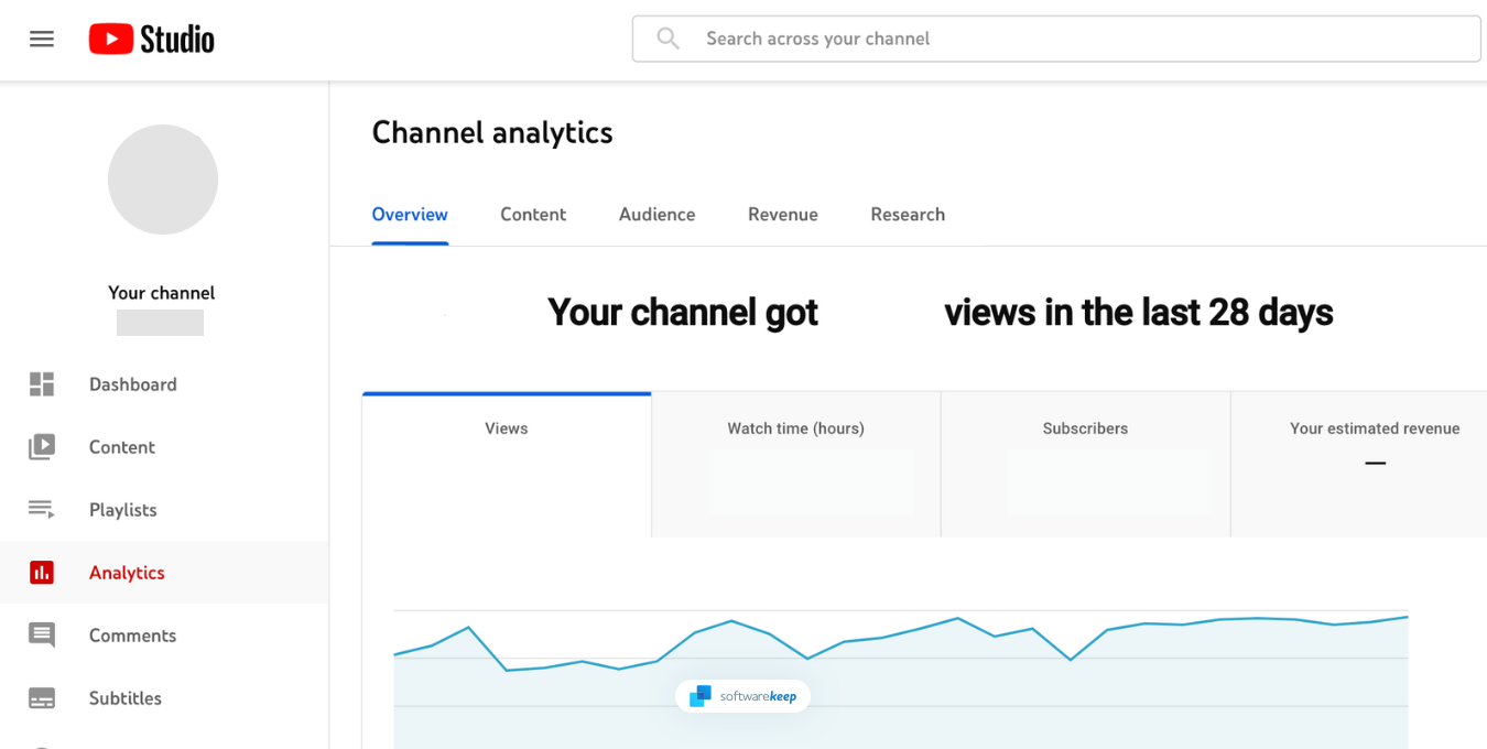
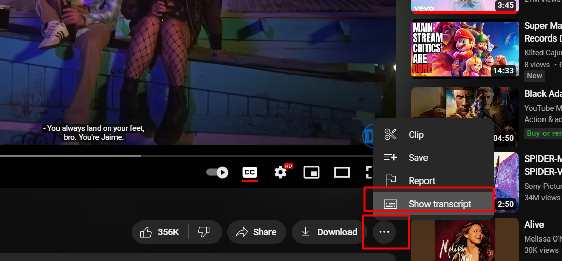
YouTube is one of the most powerful tools for affiliate marketing. With an extensive user base of over 2.68 billion individuals worldwide, YouTube allows you to reach a wide audience and create videos videos that showcase your brand, products, or services.
YouTube's advanced algorithm helps push your content out to viewers who might be interested in what you have to offer. This is a great way to start with affiliate marketing, even if you don't have an audience yet. According to data from Social Video Plaza, the average time it takes to reach 1,000 subscribers on YouTube is between 6 and 12 months. This can vary widely depending on many factors, such as the quality of your content or the frequency of your uploads.
Another great thing about Youtube is that it allows you to add affiliate links to your videos, description, comments, and channel. Having your affiliate link clearly visible makes it easy for viewers to click on them and purchase products or services from your link. For example, you can place the link as the first line of your video description or create a pinned command under it with your affiliate link.
When your YouTube content becomes more popular, the analytics will start tracking views and interactions. This data can be beneficial in finding out which strategies are creating success or need some optimization. Numerous companies look for new affiliates through YouTube channels, too. You could potentially get extra income from sponsorships and affiliate deals with an impressive analytics page.
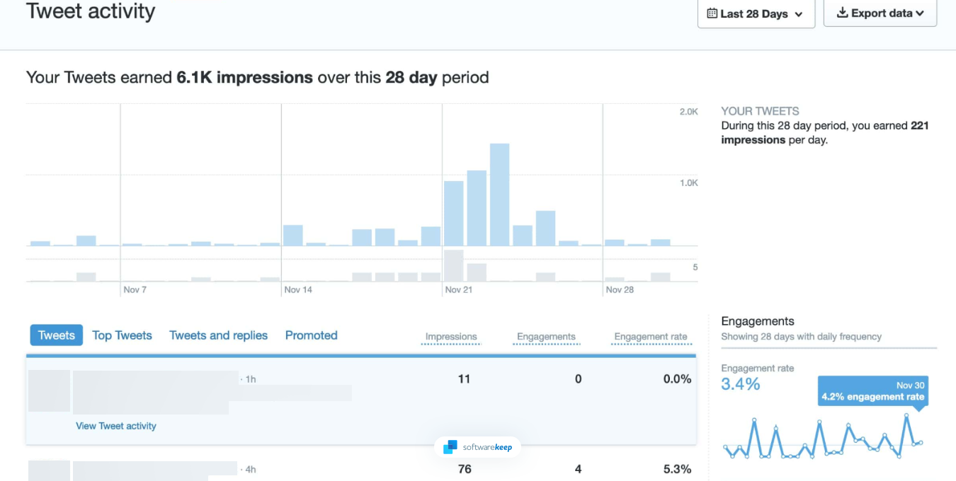
If you don't like the idea of creating videos, X (Twitter) is a perfect platform for affiliate marketing. It's highly efficient when connecting with possible clients and driving them toward your website. Despite its tight 280-character limit or more for paid X options - 4,000 characters if you have X Premium - it's still achievable to compactly communicate key points while adding value through tweets.
You can post links to blog posts, articles, or products you promote in your tweets. If your posts are missing some visuals, attaching an image or GIF is a great way to make it more attractive and eye-catching.
After you've crafted the perfect tweet, use Twitter's tools to reach your target audience quickly and check gained X or Twitter profile views. Hashtags are an effective way to gain visibility, allowing you to categorize and find related topics quickly. You can also use Twitter ads to boost specific tweets and target specific users.
Finally, X (Twitter) is an excellent platform for engaging with your followers and building relationships. If you create content that resonates with them, they're more likely to click on affiliate links placed in your tweets.
Facebook still harbors many social media users, making it an ideal platform for affiliate marketers. You can create a page and post content about your products or services. Use visuals such as photos, videos, infographics, and GIFs to make the content more attractive and engaging.
Facebook also provides helpful analytics tools for measuring engagement levels with each post. This way, you can track which strategies are working and which need improvement.
Like Twitter, hashtags can categorize content according to topics or keywords. Additionally, using Facebook ads is a great way to reach more users faster. You can target specific interests and demographics with your ad campaigns for increased visibility. To understand what kind of content resonates with your target audience, explore what your competitors are doing through the Facebook Ad Library. This will help you refine your strategy and craft even more effective ad campaigns.
You should interact with your followers frequently and nurture relationships to make the most out of Facebook. This will help strengthen the trust between yourself and your audience, making them more likely to click on affiliate links posted in your content.
Instagram offers unique tools to affiliate marketers. While the platform is heavily built on sharing images and utilizing hashtags to push out your content, you can also use Stories and Reels to promote your affiliate products in a fun and unique way. Keeping the content fresh and exciting is key to success on Instagram, as people tend to be drawn in by visuals.
Crafting captions for images to include an affiliate link can be tricky. Get creative with your approach and encourage people towards your link without being too long-winded. Asking people to check your story or bio is a popular way of placing your affiliate link in an easily accessible spot.
With Instagram stories, you can add widgets that quickly integrate a link, making it easy for your viewers to tap or click. If you have more than 10,000 followers on Instagram, you can also use the "swipe up" feature on your stories. This feature allows you to add a link that viewers can access by simply swiping up the story.
Instagram also has helpful analytics and advertising tools to measure engagement levels and reach more users quickly. Additionally, you can use influencers or collaborate with other brands to increase the visibility of your posts.
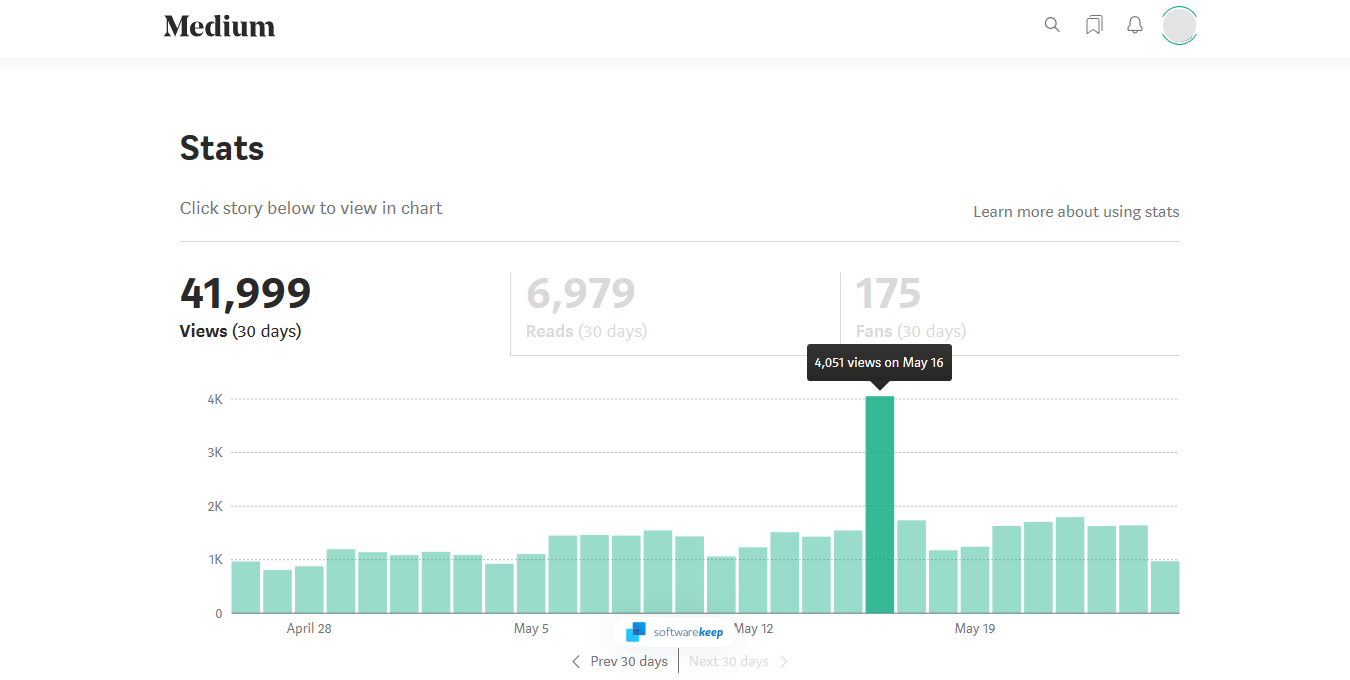
Medium is a great platform for creating content related to your chosen niche and expressing your knowledge and ideas. You can post blog articles with affiliate links and use the built-in analytics tools to measure engagement. Writing engaging, factually correct posts that give you an edge over your competitors in the same niche is important.
Using keywords and hashtags can help you reach more users on Medium, as they are used for categorizing posts according to topics or keywords. You can also use the platform's newsletter feature to send your content to a larger audience. Learning more about SEO and using the right keywords can make it easier for people to find your posts.
Medium also has its own advertising tools, which allow you to reach more users with targeted ads and track which ones are performing optimally. Additionally, you can collaborate with other authors in the same niche to increase the visibility of your posts and gain more followers.
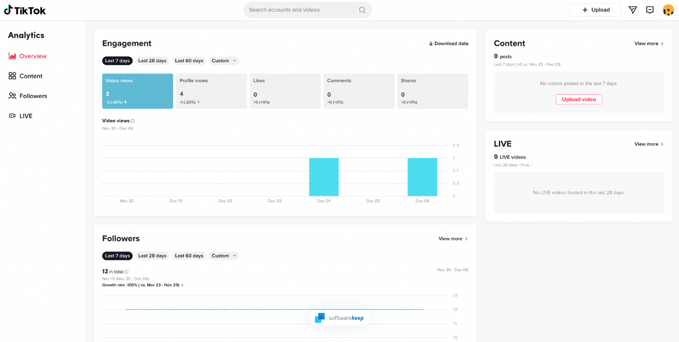
Despite its lack of credibility amongst professionals, TikTok remains one of the top social media platforms. In 2021 and 2022, global users spent around 20% more hours each month using TikTok - a clear demonstration that it is here to stay, and it's your chance to take advantage of it.
TikTok is an excellent platform for affiliates. Thanks to its advanced and always-evolving algorithm, TikTok pushes your content out to local and global audiences who might be interested in what you have to offer. Using hashtags and keyword optimization, you can also target users likely to engage with your content.
Crafting creative videos encouraging viewers to check out a link or product is key for successful affiliate marketing on TikTok. On this platform, grabbing the attention of your viewers is especially important since most videos are short clips. Using catchy and trendy music combined with creative transitions can help you capture the attention of potential customers.
Promoting your content and channel on TikTok is relatively easy. You can Maximize TikTok followers by simply interacting with other users in your niche to boost your reach and push your content out to users who interact with the same creators.
Additionally, buying TikTok likes can also enhance your content’s visibility and engagement on the platform faster. This unique feature of TikTok can help you take advantage of the platform. You can even do a live stream on TikTok to engage your audiences to buy products. In fact, you can even earn money by receiving virtual gifts like TikTok Galaxy, Lion, etc. It is a great way to not only interact with your audiences and build a strong relationship with them.
Unfortunately, you cannot place links in your video or its description on TikTok, making promoting your affiliate links tricky. We recommend creating a website or a Linktree page where you can place all your affiliate links in one place. You can then add the link to that in your TikTok bio. This way, your viewers can easily access all of your affiliate links in one place.
Creating your own website gives you the most control over your affiliate marketing efforts. You can design it to fit the needs of your target audience and customize the look and feel however you'd like. Your website is an effective platform for promoting yourself as a professional, providing information about your services or products, or publishing blog posts to get more leads.
While making a website from scratch might seem like a daunting task to take on, today's technology makes it much more accessible than ever before. With WordPress and content management systems, you can easily set up a website in no time at all and start promoting your affiliate links right away.
Once your website is up and running, several ways exist to promote your affiliate links to the right audience. You can use SEO tactics such as keyword optimization and link building to increase your website's rankings in the search engine results pages. Additionally, you can reach out to influencers or other websites in your niche and do cross-promotion activities with them.
No matter what approach you take, it is essential to remember that content is vital when it comes to successful affiliate marketing. The more engaging and informative your website content is, the more likely potential customers will click on your links and make a purchase. Quality content is essential for increasing conversion rates and achieving success with affiliate marketing.
Creating engaging content that converts requires careful planning and execution. Here are some tips to help you create content that can convert your audience into customers:
These tips can help create content that converts and increases your affiliate conversions.
Crafting engaging content is essential for successful affiliate marketers, as it increases the likelihood of reaching potential customers and converting them into buyers. When you consistently give people helpful information, they will trust you and think of you as an expert. This way, more people will buy the products or services you're affiliated with.
Here are some tips to help you use content to boost your affiliate revenue:
These tips can help you create content that converts and boosts your affiliate revenue. With a well-thought-out strategy, you can earn more money with affiliate marketing.
In conclusion, affiliate marketing can be a great way to earn money by promoting products or services that you believe in. With the rise of social media, there are many platforms that you can use to promote your affiliate links, including Instagram, YouTube, TikTok, and more. Affiliate marketing on TikTok can be a great way to grow your TikTok followers and earn money by promoting and selling other company’s products or services for a commission.
Creating engaging content and strategically sharing your affiliate links can increase the chances of driving traffic and earning commissions from your efforts. It may take some time before you start making money, but dedication to high-quality, consistent content will pay off in the long run. Good luck on your affiliate journey!
We’re glad you’ve read this article. :) Thank you for reading.
If you have a second, please share this article on your socials; someone else may benefit too.
Subscribe to our newsletter and be the first to read our future articles, reviews, and blog post right from your inbox. We also offer deals, promotions, and updates on our products and share them via email. You won’t miss one.
» How to Be a Great Affiliate
» How to Reach More People When Affiliate Marketing
» Why Be a SoftwareKeep Affiliate?
Temporary files, also known as “temp files,” for short, store data applications require to run and contain unnecessary files that can quickly fill up your disk space. In this article, we'll explore the purpose of temporary files. Find out why they exist in the first place and how you can manage them properly and free up valuable disk space for other tasks.
Temporary files are files created to temporarily hold information to free up system resources when the files aren’t needed. In Windows, temporary files can be of different types, such as installation files, log files, and backup files. These files get stored in locations depending on the type of file.
As you use your computer, temporary files are created by apps and services to hold important information temporarily. These may be cached images, videos, and other data related to the service you’re using. This practice helps retrieve the information quickly, making apps run faster.
Although they may seem unimportant, temporary files are a vital component of our computing experience, helping to keep us organized and efficient. So next time you see a temporary file, know it's serving a purpose more significant than what meets the eye.
Typically, you can find temporary files in two main locations:
If you try to access C:\Windows\Temp, you may see a message saying you don't have permission to access it. In that case, click on the "Continue" button to proceed. You'll notice that the folder contains mainly ".tmp," ".temp," and ".txt" files.
Another folder where temporary files are usually stored is C:\Users\username\AppData\Local\Temp. This folder is created for each user and is hidden by default. You must first enable "Show hidden items" from the Folder Options to see it.
The Windows operating system creates temporary files in the %system%\Windows\Temp folder, while users' temporary files created by running any software are stored in their user profiles at %userprofiles%\AppData\Local.
Sometimes, temporary files of a particular software may be in a subfolder inside the parent folder of that software. In rare cases, an app may create a temporary file or folder in the root directory of the system drive. In such a case, you should sift through the folder and delete it if you are sure it contains temporary files.
Windows temporary files exist to improve your computer's performance and ensure programs run smoothly. For example, when you open a program like Microsoft Word, it must access data stored in temporary files. So these files act as a buffer between your computer and the program, allowing you to work without significant performance lags.
In addition to optimizing your system’s performance, Windows temporary files help maintain the integrity of your documents. Whenever you save a document on Windows, a copy is stored in the temp file until that document is saved. If anything happens while saving the file (like a power failure), you can open it again using its Temp File version.
Temporary files can accumulate over time, leading to slow system performance. The accumulation can be due to various reasons, such as software installation and updates, system crashes, or even malware infections. The more temporary files accumulate, the more space they take up, which can cause the system to slow down.
Some apps do remove their temp files, but many don’t. So, keeping an eye on the temporary files and deleting them regularly to free up disk space is essential.
There are several types of Windows temporary files:
Each type of Windows temporary file serves a different purpose, and it is crucial to understand what each one does to manage them properly.
Windows temporary files can take up significant space on your hard drive if left unchecked, so it’s important to manage them properly. Here are a few tips on how to do this:
By following these tips, you can ensure that your Windows temporary files are managed correctly and that your computer is running optimally. This will free up disk space for other tasks and help keep your system performing at its best.
If you’re trying to free up some disk space and don’t need the temporary files, you can delete them quickly. There are a few ways to do this:
The most straightforward solution to clearing temporary files is manually deleting them from each folder. This involves going into the Windows Temp folder and deleting all its files.
The Settings app in Windows contains a section that allows you to clear out temporary files quickly and easily. Here's how to do it:
Storage Sense is a Windows feature that automatically deletes temporary files when your disk space runs low. To enable it, follow these steps:
You can create a BAT file to clean your temporary files automatically. BAT files are text files that you can use to execute commands. Here's how to make one:
This method is more advanced than the other options but can be helpful if you have to clear out multiple computers at once or want an automated solution for cleaning up temporary files.
The Command Prompt is a powerful tool for executing commands in Windows. You can also use it to delete temporary files quickly and easily. Here's how:
Disk Cleanup is a built-in tool in Windows that you can use to remove unnecessary files from the system. It can even delete temporary files, so it's a good idea to run it regularly to keep your disk space clutter-free. Here's how:
While Windows has a built-in tool for cleaning temporary files, third-party disk cleaners can help you do the job. These software applications are designed to scan your system for temporary files and delete them, freeing up valuable disk space and potentially improving system performance.
Here are five recommended third-party disk cleaners for deleting temporary files:
These third-party disk cleaners can help delete temporary files and other types of system junk. Just research and choose a reputable tool to avoid potential issues.
Temporary files are essential to the Windows operating system; managing them is crucial to keep your system running smoothly. By understanding what temporary files are, their types, their location, and how to manage them, you can optimize your system's performance and prevent it from slowing down. Use the best practices discussed in this article to keep your system in top shape.
We hope this article has helped you understand how temporary files work and how to manage them properly. With the right tools and practices, you can ensure your system runs optimally and free up disk space for other files.
We’re glad you’ve read this article. :) Thank you for reading.
If you have a second, please share this article on your socials; someone else may benefit too.
Subscribe to our newsletter and be the first to read our future articles, reviews, and blog post right from your inbox. We also offer deals, promotions, and updates on our products and share them via email. You won’t miss one.
» How to Find and Delete Duplicate Files in Windows 11
» How to Restore deleted files in Windows
» How to Find Large Files on Windows 10